02. Neural Network Classification with TensorFlow¶

Okay, we've seen how to deal with a regression problem in TensorFlow, let's look at how we can approach a classification problem.

A classification problem involves predicting whether something is one thing or another.

For example, you might want to:

• Predict whether or not someone has heart disease based on their health parameters. This is called binary classification since there are only two options.
• Decide whether a photo of is of food, a person or a dog. This is called multi-class classification since there are more than two options.
• Predict what categories should be assigned to a Wikipedia article. This is called multi-label classification since a single article could have more than one category assigned.

In this notebook, we're going to work through a number of different classification problems with TensorFlow. In other words, taking a set of inputs and predicting what class those set of inputs belong to.

What we're going to cover¶

Specifically, we're going to go through doing the following with TensorFlow:

• Architecture of a classification model
• Input shapes and output shapes
  • X: features/data (inputs)
  • y: labels (outputs)
    • "What class do the inputs belong to?"
• Creating custom data to view and fit
• Steps in modelling for binary and mutliclass classification
  • Creating a model
  • Compiling a model
    • Defining a loss function
    • Setting up an optimizer
      • Finding the best learning rate
    • Creating evaluation metrics
  • Fitting a model (getting it to find patterns in our data)
  • Improving a model
• The power of non-linearity
• Evaluating classification models
  • Visualizng the model ("visualize, visualize, visualize")
  • Looking at training curves
  • Compare predictions to ground truth (using our evaluation metrics)

How you can use this notebook¶

You can read through the descriptions and the code (it should all run, except for the cells which error on purpose), but there's a better option.

Write all of the code yourself.

Yes. I'm serious. Create a new notebook, and rewrite each line by yourself. Investigate it, see if you can break it, why does it break?

You don't have to write the text descriptions but writing the code yourself is a great way to get hands-on experience.

Don't worry if you make mistakes, we all do. The way to get better and make less mistakes is to write more code.

Typical architecture of a classification neural network¶

The word typical is on purpose.

Because the architecture of a classification neural network can widely vary depending on the problem you're working on.

However, there are some fundamentals all deep neural networks contain:

• An input layer.
• Some hidden layers.
• An output layer.

Much of the rest is up to the data analyst creating the model.

The following are some standard values you'll often use in your classification neural networks.

Hyperparameter	Binary Classification	Multiclass classification
Input layer shape	Same as number of features (e.g. 5 for age, sex, height, weight, smoking status in heart disease prediction)	Same as binary classification
Hidden layer(s)	Problem specific, minimum = 1, maximum = unlimited	Same as binary classification
Neurons per hidden layer	Problem specific, generally 10 to 100	Same as binary classification
Output layer shape	1 (one class or the other)	1 per class (e.g. 3 for food, person or dog photo)
Hidden activation	Usually ReLU (rectified linear unit)	Same as binary classification
Output activation	Sigmoid	Softmax
Loss function	Cross entropy (tf.keras.losses.BinaryCrossentropy in TensorFlow)	Cross entropy (tf.keras.losses.CategoricalCrossentropy in TensorFlow)
Optimizer	SGD (stochastic gradient descent), Adam	Same as binary classification

Table 1: Typical architecture of a classification network. Source: Adapted from page 295 of Hands-On Machine Learning with Scikit-Learn, Keras & TensorFlow Book by Aurélien Géron

Don't worry if not much of the above makes sense right now, we'll get plenty of experience as we go through this notebook.

Let's start by importing TensorFlow as the common alias tf. For this notebook, make sure you're using version 2.x+.

In [ ]:

import tensorflow as tf
print(tf.__version__)

import tensorflow as tf print(tf.__version__)

2.7.0

Creating data to view and fit¶

We could start by importing a classification dataset but let's practice making some of our own classification data.

🔑 Note: It's a common practice to get you and model you build working on a toy (or simple) dataset before moving to your actual problem. Treat it as a rehersal experiment before the actual experiment(s).

Since classification is predicting whether something is one thing or another, let's make some data to reflect that.

To do so, we'll use Scikit-Learn's make_circles() function.

In [ ]:

from sklearn.datasets import make_circles

# Make 1000 examples
n_samples = 1000

# Create circles
X, y = make_circles(n_samples, 
                    noise=0.03, 
                    random_state=42)

from sklearn.datasets import make_circles # Make 1000 examples n_samples = 1000 # Create circles X, y = make_circles(n_samples, noise=0.03, random_state=42)

Wonderful, now we've created some data, let's look at the features (X) and labels (y).

In [ ]:

# Check out the features
X

# Check out the features X

Out[ ]:

array([[ 0.75424625,  0.23148074],
       [-0.75615888,  0.15325888],
       [-0.81539193,  0.17328203],
       ...,
       [-0.13690036, -0.81001183],
       [ 0.67036156, -0.76750154],
       [ 0.28105665,  0.96382443]])

In [ ]:

# See the first 10 labels
y[:10]

# See the first 10 labels y[:10]

Out[ ]:

array([1, 1, 1, 1, 0, 1, 1, 1, 1, 0])

Okay, we've seen some of our data and labels, how about we move towards visualizing?

🔑 Note: One important step of starting any kind of machine learning project is to become one with the data. And one of the best ways to do this is to visualize the data you're working with as much as possible. The data explorer's motto is "visualize, visualize, visualize".

We'll start with a DataFrame.

In [ ]:

# Make dataframe of features and labels
import pandas as pd
circles = pd.DataFrame({"X0":X[:, 0], "X1":X[:, 1], "label":y})
circles.head()

# Make dataframe of features and labels import pandas as pd circles = pd.DataFrame({"X0":X[:, 0], "X1":X[:, 1], "label":y}) circles.head()

Out[ ]:

	X0	X1	label
0	0.754246	0.231481	1
1	-0.756159	0.153259	1
2	-0.815392	0.173282	1
3	-0.393731	0.692883	1
4	0.442208	-0.896723	0

What kind of labels are we dealing with?

In [ ]:

# Check out the different labels
circles.label.value_counts()

# Check out the different labels circles.label.value_counts()

Out[ ]:

1    500
0    500
Name: label, dtype: int64

Alright, looks like we're dealing with a binary classification problem. It's binary because there are only two labels (0 or 1).

If there were more label options (e.g. 0, 1, 2, 3 or 4), it would be called multiclass classification.

Let's take our visualization a step further and plot our data.

In [ ]:

# Visualize with a plot
import matplotlib.pyplot as plt
plt.scatter(X[:, 0], X[:, 1], c=y, cmap=plt.cm.RdYlBu);

# Visualize with a plot import matplotlib.pyplot as plt plt.scatter(X[:, 0], X[:, 1], c=y, cmap=plt.cm.RdYlBu);

Nice! From the plot, can you guess what kind of model we might want to build?

How about we try and build one to classify blue or red dots? As in, a model which is able to distinguish blue from red dots.

🛠 Practice: Before pushing forward, you might want to spend 10 minutes playing around with the TensorFlow Playground. Try adjusting the different hyperparameters you see and click play to see a neural network train. I think you'll find the data very similar to what we've just created.

Input and output shapes¶

One of the most common issues you'll run into when building neural networks is shape mismatches.

More specifically, the shape of the input data and the shape of the output data.

In our case, we want to input X and get our model to predict y.

So let's check out the shapes of X and y.

In [ ]:

# Check the shapes of our features and labels
X.shape, y.shape

# Check the shapes of our features and labels X.shape, y.shape

Out[ ]:

((1000, 2), (1000,))

Hmm, where do these numbers come from?

In [ ]:

# Check how many samples we have
len(X), len(y)

# Check how many samples we have len(X), len(y)

Out[ ]:

(1000, 1000)

So we've got as many X values as we do y values, that makes sense.

Let's check out one example of each.

In [ ]:

# View the first example of features and labels
X[0], y[0]

# View the first example of features and labels X[0], y[0]

Out[ ]:

(array([0.75424625, 0.23148074]), 1)

Alright, so we've got two X features which lead to one y value.

This means our neural network input shape will has to accept a tensor with at least one dimension being two and output a tensor with at least one value.

🤔 Note: y having a shape of (1000,) can seem confusing. However, this is because all y values are actually scalars (single values) and therefore don't have a dimension. For now, think of your output shape as being at least the same value as one example of y (in our case, the output from our neural network has to be at least one value).

Steps in modelling¶

Now we know what data we have as well as the input and output shapes, let's see how we'd build a neural network to model it.

In TensorFlow, there are typically 3 fundamental steps to creating and training a model.

1. Creating a model - piece together the layers of a neural network yourself (using the functional or sequential API) or import a previously built model (known as transfer learning).
2. Compiling a model - defining how a model's performance should be measured (loss/metrics) as well as defining how it should improve (optimizer).
3. Fitting a model - letting the model try to find patterns in the data (how does X get to y).

Let's see these in action using the Sequential API to build a model for our regression data. And then we'll step through each.

In [ ]:

# Set random seed
tf.random.set_seed(42)

# 1. Create the model using the Sequential API
model_1 = tf.keras.Sequential([
  tf.keras.layers.Dense(1)
])

# 2. Compile the model
model_1.compile(loss=tf.keras.losses.BinaryCrossentropy(), # binary since we are working with 2 clases (0 & 1)
                optimizer=tf.keras.optimizers.SGD(),
                metrics=['accuracy'])

# 3. Fit the model
model_1.fit(X, y, epochs=5)

# Set random seed tf.random.set_seed(42) # 1. Create the model using the Sequential API model_1 = tf.keras.Sequential([ tf.keras.layers.Dense(1) ]) # 2. Compile the model model_1.compile(loss=tf.keras.losses.BinaryCrossentropy(), # binary since we are working with 2 clases (0 & 1) optimizer=tf.keras.optimizers.SGD(), metrics=['accuracy']) # 3. Fit the model model_1.fit(X, y, epochs=5)

Epoch 1/5
32/32 [==============================] - 1s 2ms/step - loss: 2.8544 - accuracy: 0.4600
Epoch 2/5
32/32 [==============================] - 0s 2ms/step - loss: 0.7131 - accuracy: 0.5430
Epoch 3/5
32/32 [==============================] - 0s 1ms/step - loss: 0.6973 - accuracy: 0.5090
Epoch 4/5
32/32 [==============================] - 0s 1ms/step - loss: 0.6950 - accuracy: 0.5010
Epoch 5/5
32/32 [==============================] - 0s 1ms/step - loss: 0.6942 - accuracy: 0.4830

Out[ ]:

<keras.callbacks.History at 0x7ff186346190>

Looking at the accuracy metric, our model performs poorly (50% accuracy on a binary classification problem is the equivalent of guessing), but what if we trained it for longer?

In [ ]:

# Train our model for longer (more chances to look at the data)
model_1.fit(X, y, epochs=200, verbose=0) # set verbose=0 to remove training updates
model_1.evaluate(X, y)

# Train our model for longer (more chances to look at the data) model_1.fit(X, y, epochs=200, verbose=0) # set verbose=0 to remove training updates model_1.evaluate(X, y)

32/32 [==============================] - 0s 2ms/step - loss: 0.6935 - accuracy: 0.5000

Out[ ]:

[0.6934829950332642, 0.5]

Even after 200 passes of the data, it's still performing as if it's guessing.

What if we added an extra layer and trained for a little longer?

In [ ]:

# Set random seed
tf.random.set_seed(42)

# 1. Create the model (same as model_1 but with an extra layer)
model_2 = tf.keras.Sequential([
  tf.keras.layers.Dense(1), # add an extra layer
  tf.keras.layers.Dense(1) 
])

# 2. Compile the model
model_2.compile(loss=tf.keras.losses.BinaryCrossentropy(),
                optimizer=tf.keras.optimizers.SGD(),
                metrics=['accuracy'])

# 3. Fit the model
model_2.fit(X, y, epochs=100, verbose=0) # set verbose=0 to make the output print less

# Set random seed tf.random.set_seed(42) # 1. Create the model (same as model_1 but with an extra layer) model_2 = tf.keras.Sequential([ tf.keras.layers.Dense(1), # add an extra layer tf.keras.layers.Dense(1) ]) # 2. Compile the model model_2.compile(loss=tf.keras.losses.BinaryCrossentropy(), optimizer=tf.keras.optimizers.SGD(), metrics=['accuracy']) # 3. Fit the model model_2.fit(X, y, epochs=100, verbose=0) # set verbose=0 to make the output print less

Out[ ]:

<keras.callbacks.History at 0x7ff18496b710>

In [ ]:

# Evaluate the model
model_2.evaluate(X, y)

# Evaluate the model model_2.evaluate(X, y)

32/32 [==============================] - 0s 2ms/step - loss: 0.6933 - accuracy: 0.5000

Out[ ]:

[0.6933314800262451, 0.5]

Still not even as good as guessing (~50% accuracy)... hmm...?

Let's remind ourselves of a couple more ways we can use to improve our models.

Improving a model¶

To improve our model, we can alter almost every part of the 3 steps we went through before.

1. Creating a model - here you might want to add more layers, increase the number of hidden units (also called neurons) within each layer, change the activation functions of each layer.
2. Compiling a model - you might want to choose a different optimization function (such as the Adam optimizer, which is usually pretty good for many problems) or perhaps change the learning rate of the optimization function.
3. Fitting a model - perhaps you could fit a model for more epochs (leave it training for longer).

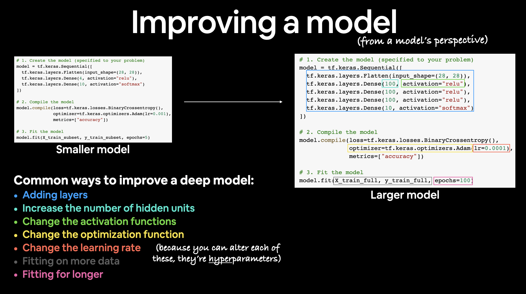There are many different ways to potentially improve a neural network. Some of the most common include: increasing the number of layers (making the network deeper), increasing the number of hidden units (making the network wider) and changing the learning rate. Because these values are all human-changeable, they're referred to as hyperparameters) and the practice of trying to find the best hyperparameters is referred to as hyperparameter tuning.

How about we try adding more neurons, an extra layer and our friend the Adam optimizer?

Surely doing this will result in predictions better than guessing...

Note: If you're using TensorFlow 2.7.0+ the original code from the following cells may have caused some errors. They've since been updated to fix those errors. You can see explanations on what happened at the following resources:

• Example Colab Notebook
• TensorFlow for Deep Learning GitHub Discussion on TensorFlow 2.7.0 breaking changes

In [ ]:

# Set random seed
tf.random.set_seed(42)

# 1. Create the model (this time 3 layers)
model_3 = tf.keras.Sequential([
  # Before TensorFlow 2.7.0
  # tf.keras.layers.Dense(100), # add 100 dense neurons

  ## After TensorFlow 2.7.0 ##
  tf.keras.layers.Dense(100, input_shape=(None, 1)), # add 100 dense neurons with input_shape defined (None, 1) = look at 1 sample at a time
  tf.keras.layers.Dense(10), # add another layer with 10 neurons
  tf.keras.layers.Dense(1)
])

# 2. Compile the model
model_3.compile(loss=tf.keras.losses.BinaryCrossentropy(),
                optimizer=tf.keras.optimizers.Adam(), # use Adam instead of SGD
                metrics=['accuracy'])

# 3. Fit the model
model_3.fit(X, y, epochs=100, verbose=0) # fit for 100 passes of the data

# Set random seed tf.random.set_seed(42) # 1. Create the model (this time 3 layers) model_3 = tf.keras.Sequential([ # Before TensorFlow 2.7.0 # tf.keras.layers.Dense(100), # add 100 dense neurons ## After TensorFlow 2.7.0 ## tf.keras.layers.Dense(100, input_shape=(None, 1)), # add 100 dense neurons with input_shape defined (None, 1) = look at 1 sample at a time tf.keras.layers.Dense(10), # add another layer with 10 neurons tf.keras.layers.Dense(1) ]) # 2. Compile the model model_3.compile(loss=tf.keras.losses.BinaryCrossentropy(), optimizer=tf.keras.optimizers.Adam(), # use Adam instead of SGD metrics=['accuracy']) # 3. Fit the model model_3.fit(X, y, epochs=100, verbose=0) # fit for 100 passes of the data

Out[ ]:

<keras.callbacks.History at 0x7ff186166e10>

Still!

We've pulled out a few tricks but our model isn't even doing better than guessing.

Let's make some visualizations to see what's happening.

🔑 Note: Whenever your model is performing strangely or there's something going on with your data you're not quite sure of, remember these three words: visualize, visualize, visualize. Inspect your data, inspect your model, inpsect your model's predictions.

To visualize our model's predictions we're going to create a function plot_decision_boundary() which:

• Takes in a trained model, features (X) and labels (y).
• Creates a meshgrid of the different X values.
• Makes predictions across the meshgrid.
• Plots the predictions as well as a line between the different zones (where each unique class falls).

If this sounds confusing, let's see it in code and then see the output.

🔑 Note: If you're ever unsure of what a function does, try unraveling it and writing it line by line for yourself to see what it does. Break it into small parts and see what each part outputs.

In [ ]:

import numpy as np

def plot_decision_boundary(model, X, y):
  """
  Plots the decision boundary created by a model predicting on X.
  This function has been adapted from two phenomenal resources:
   1. CS231n - https://cs231n.github.io/neural-networks-case-study/
   2. Made with ML basics - https://github.com/GokuMohandas/MadeWithML/blob/main/notebooks/08_Neural_Networks.ipynb
  """
  # Define the axis boundaries of the plot and create a meshgrid
  x_min, x_max = X[:, 0].min() - 0.1, X[:, 0].max() + 0.1
  y_min, y_max = X[:, 1].min() - 0.1, X[:, 1].max() + 0.1
  xx, yy = np.meshgrid(np.linspace(x_min, x_max, 100),
                       np.linspace(y_min, y_max, 100))
  
  # Create X values (we're going to predict on all of these)
  x_in = np.c_[xx.ravel(), yy.ravel()] # stack 2D arrays together: https://numpy.org/devdocs/reference/generated/numpy.c_.html
  
  # Make predictions using the trained model
  y_pred = model.predict(x_in)

  # Check for multi-class
  if len(y_pred[0]) > 1:
    print("doing multiclass classification...")
    # We have to reshape our predictions to get them ready for plotting
    y_pred = np.argmax(y_pred, axis=1).reshape(xx.shape)
  else:
    print("doing binary classifcation...")
    y_pred = np.round(y_pred).reshape(xx.shape)
  
  # Plot decision boundary
  plt.contourf(xx, yy, y_pred, cmap=plt.cm.RdYlBu, alpha=0.7)
  plt.scatter(X[:, 0], X[:, 1], c=y, s=40, cmap=plt.cm.RdYlBu)
  plt.xlim(xx.min(), xx.max())
  plt.ylim(yy.min(), yy.max())

import numpy as np def plot_decision_boundary(model, X, y): """ Plots the decision boundary created by a model predicting on X. This function has been adapted from two phenomenal resources: 1. CS231n - https://cs231n.github.io/neural-networks-case-study/ 2. Made with ML basics - https://github.com/GokuMohandas/MadeWithML/blob/main/notebooks/08_Neural_Networks.ipynb """ # Define the axis boundaries of the plot and create a meshgrid x_min, x_max = X[:, 0].min() - 0.1, X[:, 0].max() + 0.1 y_min, y_max = X[:, 1].min() - 0.1, X[:, 1].max() + 0.1 xx, yy = np.meshgrid(np.linspace(x_min, x_max, 100), np.linspace(y_min, y_max, 100)) # Create X values (we're going to predict on all of these) x_in = np.c_[xx.ravel(), yy.ravel()] # stack 2D arrays together: https://numpy.org/devdocs/reference/generated/numpy.c_.html # Make predictions using the trained model y_pred = model.predict(x_in) # Check for multi-class if len(y_pred[0]) > 1: print("doing multiclass classification...") # We have to reshape our predictions to get them ready for plotting y_pred = np.argmax(y_pred, axis=1).reshape(xx.shape) else: print("doing binary classifcation...") y_pred = np.round(y_pred).reshape(xx.shape) # Plot decision boundary plt.contourf(xx, yy, y_pred, cmap=plt.cm.RdYlBu, alpha=0.7) plt.scatter(X[:, 0], X[:, 1], c=y, s=40, cmap=plt.cm.RdYlBu) plt.xlim(xx.min(), xx.max()) plt.ylim(yy.min(), yy.max())

Now we've got a function to plot our model's decision boundary (the cut off point its making between red and blue dots), let's try it out.

In [ ]:

# Check out the predictions our model is making 
plot_decision_boundary(model_3, X, y)

# Check out the predictions our model is making plot_decision_boundary(model_3, X, y)

doing multiclass classification...

Looks like our model is trying to draw a straight line through the data.

What's wrong with doing this?

The main issue is our data isn't separable by a straight line.

In a regression problem, our model might work. In fact, let's try it.

In [ ]:

# Set random seed
tf.random.set_seed(42)

# Create some regression data
X_regression = np.arange(0, 1000, 5)
y_regression = np.arange(100, 1100, 5)

# Split it into training and test sets
X_reg_train = X_regression[:150]
X_reg_test = X_regression[150:]
y_reg_train = y_regression[:150]
y_reg_test = y_regression[150:]

# Fit our model to the data
# Note: Before TensorFlow 2.7.0, this line would work
# model_3.fit(X_reg_train, y_reg_train, epochs=100)

# After TensorFlow 2.7.0, see here for more: https://github.com/mrdbourke/tensorflow-deep-learning/discussions/278
model_3.fit(tf.expand_dims(X_reg_train, axis=-1), 
            y_reg_train,
            epochs=100)

# Set random seed tf.random.set_seed(42) # Create some regression data X_regression = np.arange(0, 1000, 5) y_regression = np.arange(100, 1100, 5) # Split it into training and test sets X_reg_train = X_regression[:150] X_reg_test = X_regression[150:] y_reg_train = y_regression[:150] y_reg_test = y_regression[150:] # Fit our model to the data # Note: Before TensorFlow 2.7.0, this line would work # model_3.fit(X_reg_train, y_reg_train, epochs=100) # After TensorFlow 2.7.0, see here for more: https://github.com/mrdbourke/tensorflow-deep-learning/discussions/278 model_3.fit(tf.expand_dims(X_reg_train, axis=-1), y_reg_train, epochs=100)

Epoch 1/100
5/5 [==============================] - 0s 4ms/step - loss: -4016.9167 - accuracy: 0.0000e+00
Epoch 2/100
5/5 [==============================] - 0s 4ms/step - loss: -7145.1201 - accuracy: 0.0000e+00
Epoch 3/100
5/5 [==============================] - 0s 3ms/step - loss: -7154.2476 - accuracy: 0.0000e+00
Epoch 4/100
5/5 [==============================] - 0s 4ms/step - loss: -7190.0156 - accuracy: 0.0000e+00
Epoch 5/100
5/5 [==============================] - 0s 4ms/step - loss: -7190.0156 - accuracy: 0.0000e+00
Epoch 6/100
5/5 [==============================] - 0s 4ms/step - loss: -7190.0156 - accuracy: 0.0000e+00
Epoch 7/100
5/5 [==============================] - 0s 4ms/step - loss: -7190.0156 - accuracy: 0.0000e+00
Epoch 8/100
5/5 [==============================] - 0s 5ms/step - loss: -7190.0156 - accuracy: 0.0000e+00
Epoch 9/100
5/5 [==============================] - 0s 4ms/step - loss: -7190.0156 - accuracy: 0.0000e+00
Epoch 10/100
5/5 [==============================] - 0s 4ms/step - loss: -7190.0156 - accuracy: 0.0000e+00
Epoch 11/100
5/5 [==============================] - 0s 5ms/step - loss: -7190.0156 - accuracy: 0.0000e+00
Epoch 12/100
5/5 [==============================] - 0s 5ms/step - loss: -7190.0156 - accuracy: 0.0000e+00
Epoch 13/100
5/5 [==============================] - 0s 3ms/step - loss: -7190.0156 - accuracy: 0.0000e+00
Epoch 14/100
5/5 [==============================] - 0s 4ms/step - loss: -7190.0156 - accuracy: 0.0000e+00
Epoch 15/100
5/5 [==============================] - 0s 4ms/step - loss: -7190.0156 - accuracy: 0.0000e+00
Epoch 16/100
5/5 [==============================] - 0s 4ms/step - loss: -7190.0156 - accuracy: 0.0000e+00
Epoch 17/100
5/5 [==============================] - 0s 4ms/step - loss: -7190.0156 - accuracy: 0.0000e+00
Epoch 18/100
5/5 [==============================] - 0s 3ms/step - loss: -7190.0151 - accuracy: 0.0000e+00
Epoch 19/100
5/5 [==============================] - 0s 5ms/step - loss: -7190.0151 - accuracy: 0.0000e+00
Epoch 20/100
5/5 [==============================] - 0s 4ms/step - loss: -7190.0156 - accuracy: 0.0000e+00
Epoch 21/100
5/5 [==============================] - 0s 5ms/step - loss: -7190.0156 - accuracy: 0.0000e+00
Epoch 22/100
5/5 [==============================] - 0s 4ms/step - loss: -7190.0156 - accuracy: 0.0000e+00
Epoch 23/100
5/5 [==============================] - 0s 4ms/step - loss: -7190.0156 - accuracy: 0.0000e+00
Epoch 24/100
5/5 [==============================] - 0s 5ms/step - loss: -7190.0151 - accuracy: 0.0000e+00
Epoch 25/100
5/5 [==============================] - 0s 3ms/step - loss: -7190.0156 - accuracy: 0.0000e+00
Epoch 26/100
5/5 [==============================] - 0s 5ms/step - loss: -7190.0156 - accuracy: 0.0000e+00
Epoch 27/100
5/5 [==============================] - 0s 4ms/step - loss: -7190.0151 - accuracy: 0.0000e+00
Epoch 28/100
5/5 [==============================] - 0s 4ms/step - loss: -7190.0156 - accuracy: 0.0000e+00
Epoch 29/100
5/5 [==============================] - 0s 5ms/step - loss: -7190.0156 - accuracy: 0.0000e+00
Epoch 30/100
5/5 [==============================] - 0s 4ms/step - loss: -7190.0156 - accuracy: 0.0000e+00
Epoch 31/100
5/5 [==============================] - 0s 4ms/step - loss: -7190.0156 - accuracy: 0.0000e+00
Epoch 32/100
5/5 [==============================] - 0s 5ms/step - loss: -7190.0156 - accuracy: 0.0000e+00
Epoch 33/100
5/5 [==============================] - 0s 4ms/step - loss: -7190.0156 - accuracy: 0.0000e+00
Epoch 34/100
5/5 [==============================] - 0s 5ms/step - loss: -7190.0156 - accuracy: 0.0000e+00
Epoch 35/100
5/5 [==============================] - 0s 4ms/step - loss: -7190.0156 - accuracy: 0.0000e+00
Epoch 36/100
5/5 [==============================] - 0s 4ms/step - loss: -7190.0151 - accuracy: 0.0000e+00
Epoch 37/100
5/5 [==============================] - 0s 7ms/step - loss: -7190.0156 - accuracy: 0.0000e+00
Epoch 38/100
5/5 [==============================] - 0s 4ms/step - loss: -7190.0156 - accuracy: 0.0000e+00
Epoch 39/100
5/5 [==============================] - 0s 5ms/step - loss: -7190.0151 - accuracy: 0.0000e+00
Epoch 40/100
5/5 [==============================] - 0s 5ms/step - loss: -7190.0156 - accuracy: 0.0000e+00
Epoch 41/100
5/5 [==============================] - 0s 5ms/step - loss: -7190.0156 - accuracy: 0.0000e+00
Epoch 42/100
5/5 [==============================] - 0s 5ms/step - loss: -7190.0156 - accuracy: 0.0000e+00
Epoch 43/100
5/5 [==============================] - 0s 4ms/step - loss: -7190.0156 - accuracy: 0.0000e+00
Epoch 44/100
5/5 [==============================] - 0s 5ms/step - loss: -7190.0156 - accuracy: 0.0000e+00
Epoch 45/100
5/5 [==============================] - 0s 4ms/step - loss: -7190.0156 - accuracy: 0.0000e+00
Epoch 46/100
5/5 [==============================] - 0s 4ms/step - loss: -7190.0156 - accuracy: 0.0000e+00
Epoch 47/100
5/5 [==============================] - 0s 4ms/step - loss: -7190.0156 - accuracy: 0.0000e+00
Epoch 48/100
5/5 [==============================] - 0s 4ms/step - loss: -7190.0156 - accuracy: 0.0000e+00
Epoch 49/100
5/5 [==============================] - 0s 4ms/step - loss: -7190.0156 - accuracy: 0.0000e+00
Epoch 50/100
5/5 [==============================] - 0s 4ms/step - loss: -7190.0156 - accuracy: 0.0000e+00
Epoch 51/100
5/5 [==============================] - 0s 4ms/step - loss: -7190.0156 - accuracy: 0.0000e+00
Epoch 52/100
5/5 [==============================] - 0s 5ms/step - loss: -7190.0156 - accuracy: 0.0000e+00
Epoch 53/100
5/5 [==============================] - 0s 5ms/step - loss: -7190.0156 - accuracy: 0.0000e+00
Epoch 54/100
5/5 [==============================] - 0s 4ms/step - loss: -7190.0156 - accuracy: 0.0000e+00
Epoch 55/100
5/5 [==============================] - 0s 4ms/step - loss: -7190.0156 - accuracy: 0.0000e+00
Epoch 56/100
5/5 [==============================] - 0s 7ms/step - loss: -7190.0156 - accuracy: 0.0000e+00
Epoch 57/100
5/5 [==============================] - 0s 4ms/step - loss: -7190.0156 - accuracy: 0.0000e+00
Epoch 58/100
5/5 [==============================] - 0s 4ms/step - loss: -7190.0156 - accuracy: 0.0000e+00
Epoch 59/100
5/5 [==============================] - 0s 4ms/step - loss: -7190.0156 - accuracy: 0.0000e+00
Epoch 60/100
5/5 [==============================] - 0s 4ms/step - loss: -7190.0156 - accuracy: 0.0000e+00
Epoch 61/100
5/5 [==============================] - 0s 4ms/step - loss: -7190.0156 - accuracy: 0.0000e+00
Epoch 62/100
5/5 [==============================] - 0s 4ms/step - loss: -7190.0151 - accuracy: 0.0000e+00
Epoch 63/100
5/5 [==============================] - 0s 4ms/step - loss: -7190.0156 - accuracy: 0.0000e+00
Epoch 64/100
5/5 [==============================] - 0s 4ms/step - loss: -7190.0156 - accuracy: 0.0000e+00
Epoch 65/100
5/5 [==============================] - 0s 6ms/step - loss: -7190.0156 - accuracy: 0.0000e+00
Epoch 66/100
5/5 [==============================] - 0s 5ms/step - loss: -7190.0156 - accuracy: 0.0000e+00
Epoch 67/100
5/5 [==============================] - 0s 5ms/step - loss: -7190.0156 - accuracy: 0.0000e+00
Epoch 68/100
5/5 [==============================] - 0s 4ms/step - loss: -7190.0156 - accuracy: 0.0000e+00
Epoch 69/100
5/5 [==============================] - 0s 4ms/step - loss: -7190.0156 - accuracy: 0.0000e+00
Epoch 70/100
5/5 [==============================] - 0s 5ms/step - loss: -7190.0156 - accuracy: 0.0000e+00
Epoch 71/100
5/5 [==============================] - 0s 5ms/step - loss: -7190.0156 - accuracy: 0.0000e+00
Epoch 72/100
5/5 [==============================] - 0s 4ms/step - loss: -7190.0156 - accuracy: 0.0000e+00
Epoch 73/100
5/5 [==============================] - 0s 4ms/step - loss: -7190.0156 - accuracy: 0.0000e+00
Epoch 74/100
5/5 [==============================] - 0s 5ms/step - loss: -7190.0156 - accuracy: 0.0000e+00
Epoch 75/100
5/5 [==============================] - 0s 4ms/step - loss: -7190.0156 - accuracy: 0.0000e+00
Epoch 76/100
5/5 [==============================] - 0s 4ms/step - loss: -7190.0156 - accuracy: 0.0000e+00
Epoch 77/100
5/5 [==============================] - 0s 4ms/step - loss: -7190.0156 - accuracy: 0.0000e+00
Epoch 78/100
5/5 [==============================] - 0s 5ms/step - loss: -7190.0156 - accuracy: 0.0000e+00
Epoch 79/100
5/5 [==============================] - 0s 4ms/step - loss: -7190.0151 - accuracy: 0.0000e+00
Epoch 80/100
5/5 [==============================] - 0s 5ms/step - loss: -7190.0151 - accuracy: 0.0000e+00
Epoch 81/100
5/5 [==============================] - 0s 4ms/step - loss: -7190.0156 - accuracy: 0.0000e+00
Epoch 82/100
5/5 [==============================] - 0s 5ms/step - loss: -7190.0166 - accuracy: 0.0000e+00
Epoch 83/100
5/5 [==============================] - 0s 5ms/step - loss: -7190.0156 - accuracy: 0.0000e+00
Epoch 84/100
5/5 [==============================] - 0s 4ms/step - loss: -7190.0156 - accuracy: 0.0000e+00
Epoch 85/100
5/5 [==============================] - 0s 4ms/step - loss: -7190.0166 - accuracy: 0.0000e+00
Epoch 86/100
5/5 [==============================] - 0s 4ms/step - loss: -7190.0156 - accuracy: 0.0000e+00
Epoch 87/100
5/5 [==============================] - 0s 5ms/step - loss: -7190.0156 - accuracy: 0.0000e+00
Epoch 88/100
5/5 [==============================] - 0s 4ms/step - loss: -7190.0156 - accuracy: 0.0000e+00
Epoch 89/100
5/5 [==============================] - 0s 5ms/step - loss: -7190.0156 - accuracy: 0.0000e+00
Epoch 90/100
5/5 [==============================] - 0s 4ms/step - loss: -7190.0156 - accuracy: 0.0000e+00
Epoch 91/100
5/5 [==============================] - 0s 7ms/step - loss: -7190.0151 - accuracy: 0.0000e+00
Epoch 92/100
5/5 [==============================] - 0s 5ms/step - loss: -7190.0156 - accuracy: 0.0000e+00
Epoch 93/100
5/5 [==============================] - 0s 4ms/step - loss: -7190.0156 - accuracy: 0.0000e+00
Epoch 94/100
5/5 [==============================] - 0s 5ms/step - loss: -7190.0156 - accuracy: 0.0000e+00
Epoch 95/100
5/5 [==============================] - 0s 4ms/step - loss: -7190.0156 - accuracy: 0.0000e+00
Epoch 96/100
5/5 [==============================] - 0s 5ms/step - loss: -7190.0151 - accuracy: 0.0000e+00
Epoch 97/100
5/5 [==============================] - 0s 4ms/step - loss: -7190.0156 - accuracy: 0.0000e+00
Epoch 98/100
5/5 [==============================] - 0s 4ms/step - loss: -7190.0156 - accuracy: 0.0000e+00
Epoch 99/100
5/5 [==============================] - 0s 4ms/step - loss: -7190.0156 - accuracy: 0.0000e+00
Epoch 100/100
5/5 [==============================] - 0s 4ms/step - loss: -7190.0156 - accuracy: 0.0000e+00

Out[ ]:

<keras.callbacks.History at 0x7ff1859c4d50>

In [ ]:

model_3.summary()

model_3.summary()

Model: "sequential_2"
_________________________________________________________________
 Layer (type)                Output Shape              Param #   
=================================================================
 dense_3 (Dense)             (None, None, 100)         200       
                                                                 
 dense_4 (Dense)             (None, None, 10)          1010      
                                                                 
 dense_5 (Dense)             (None, None, 1)           11        
                                                                 
=================================================================
Total params: 1,221
Trainable params: 1,221
Non-trainable params: 0
_________________________________________________________________

Oh wait... we compiled our model for a binary classification problem.

No trouble, we can recreate it for a regression problem.

In [ ]:

# Setup random seed
tf.random.set_seed(42)

# Recreate the model
model_3 = tf.keras.Sequential([
  tf.keras.layers.Dense(100),
  tf.keras.layers.Dense(10),
  tf.keras.layers.Dense(1)
])

# Change the loss and metrics of our compiled model
model_3.compile(loss=tf.keras.losses.mae, # change the loss function to be regression-specific
                optimizer=tf.keras.optimizers.Adam(),
                metrics=['mae']) # change the metric to be regression-specific

# Fit the recompiled model
model_3.fit(tf.expand_dims(X_reg_train, axis=-1), 
            y_reg_train, 
            epochs=100)

# Setup random seed tf.random.set_seed(42) # Recreate the model model_3 = tf.keras.Sequential([ tf.keras.layers.Dense(100), tf.keras.layers.Dense(10), tf.keras.layers.Dense(1) ]) # Change the loss and metrics of our compiled model model_3.compile(loss=tf.keras.losses.mae, # change the loss function to be regression-specific optimizer=tf.keras.optimizers.Adam(), metrics=['mae']) # change the metric to be regression-specific # Fit the recompiled model model_3.fit(tf.expand_dims(X_reg_train, axis=-1), y_reg_train, epochs=100)

Epoch 1/100
5/5 [==============================] - 0s 3ms/step - loss: 248.2155 - mae: 248.2155
Epoch 2/100
5/5 [==============================] - 0s 3ms/step - loss: 138.9005 - mae: 138.9005
Epoch 3/100
5/5 [==============================] - 0s 3ms/step - loss: 53.1039 - mae: 53.1039
Epoch 4/100
5/5 [==============================] - 0s 3ms/step - loss: 73.5170 - mae: 73.5170
Epoch 5/100
5/5 [==============================] - 0s 3ms/step - loss: 71.2358 - mae: 71.2358
Epoch 6/100
5/5 [==============================] - 0s 3ms/step - loss: 47.0040 - mae: 47.0040
Epoch 7/100
5/5 [==============================] - 0s 4ms/step - loss: 45.9386 - mae: 45.9386
Epoch 8/100
5/5 [==============================] - 0s 4ms/step - loss: 42.3638 - mae: 42.3638
Epoch 9/100
5/5 [==============================] - 0s 4ms/step - loss: 43.6831 - mae: 43.6831
Epoch 10/100
5/5 [==============================] - 0s 4ms/step - loss: 42.6198 - mae: 42.6198
Epoch 11/100
5/5 [==============================] - 0s 4ms/step - loss: 42.4797 - mae: 42.4797
Epoch 12/100
5/5 [==============================] - 0s 3ms/step - loss: 41.5537 - mae: 41.5537
Epoch 13/100
5/5 [==============================] - 0s 4ms/step - loss: 42.0972 - mae: 42.0972
Epoch 14/100
5/5 [==============================] - 0s 4ms/step - loss: 41.8647 - mae: 41.8647
Epoch 15/100
5/5 [==============================] - 0s 4ms/step - loss: 41.5342 - mae: 41.5342
Epoch 16/100
5/5 [==============================] - 0s 4ms/step - loss: 41.4028 - mae: 41.4028
Epoch 17/100
5/5 [==============================] - 0s 4ms/step - loss: 41.6887 - mae: 41.6887
Epoch 18/100
5/5 [==============================] - 0s 4ms/step - loss: 41.6137 - mae: 41.6137
Epoch 19/100
5/5 [==============================] - 0s 4ms/step - loss: 41.2796 - mae: 41.2796
Epoch 20/100
5/5 [==============================] - 0s 4ms/step - loss: 41.1947 - mae: 41.1947
Epoch 21/100
5/5 [==============================] - 0s 4ms/step - loss: 41.2130 - mae: 41.2130
Epoch 22/100
5/5 [==============================] - 0s 6ms/step - loss: 41.0893 - mae: 41.0893
Epoch 23/100
5/5 [==============================] - 0s 4ms/step - loss: 41.2019 - mae: 41.2019
Epoch 24/100
5/5 [==============================] - 0s 3ms/step - loss: 40.9989 - mae: 40.9989
Epoch 25/100
5/5 [==============================] - 0s 3ms/step - loss: 41.0131 - mae: 41.0131
Epoch 26/100
5/5 [==============================] - 0s 3ms/step - loss: 41.0654 - mae: 41.0654
Epoch 27/100
5/5 [==============================] - 0s 3ms/step - loss: 40.8764 - mae: 40.8764
Epoch 28/100
5/5 [==============================] - 0s 3ms/step - loss: 41.0545 - mae: 41.0545
Epoch 29/100
5/5 [==============================] - 0s 3ms/step - loss: 41.0480 - mae: 41.0480
Epoch 30/100
5/5 [==============================] - 0s 3ms/step - loss: 40.8807 - mae: 40.8807
Epoch 31/100
5/5 [==============================] - 0s 3ms/step - loss: 41.2695 - mae: 41.2695
Epoch 32/100
5/5 [==============================] - 0s 3ms/step - loss: 40.9949 - mae: 40.9949
Epoch 33/100
5/5 [==============================] - 0s 3ms/step - loss: 41.0760 - mae: 41.0760
Epoch 34/100
5/5 [==============================] - 0s 3ms/step - loss: 41.2471 - mae: 41.2471
Epoch 35/100
5/5 [==============================] - 0s 3ms/step - loss: 40.6102 - mae: 40.6102
Epoch 36/100
5/5 [==============================] - 0s 3ms/step - loss: 41.1093 - mae: 41.1093
Epoch 37/100
5/5 [==============================] - 0s 4ms/step - loss: 40.8191 - mae: 40.8191
Epoch 38/100
5/5 [==============================] - 0s 5ms/step - loss: 40.2485 - mae: 40.2485
Epoch 39/100
5/5 [==============================] - 0s 4ms/step - loss: 41.0625 - mae: 41.0625
Epoch 40/100
5/5 [==============================] - 0s 4ms/step - loss: 40.5311 - mae: 40.5311
Epoch 41/100
5/5 [==============================] - 0s 3ms/step - loss: 40.5497 - mae: 40.5497
Epoch 42/100
5/5 [==============================] - 0s 4ms/step - loss: 40.4322 - mae: 40.4322
Epoch 43/100
5/5 [==============================] - 0s 4ms/step - loss: 40.5367 - mae: 40.5367
Epoch 44/100
5/5 [==============================] - 0s 5ms/step - loss: 40.2487 - mae: 40.2487
Epoch 45/100
5/5 [==============================] - 0s 3ms/step - loss: 40.5152 - mae: 40.5152
Epoch 46/100
5/5 [==============================] - 0s 3ms/step - loss: 40.3702 - mae: 40.3702
Epoch 47/100
5/5 [==============================] - 0s 4ms/step - loss: 40.4769 - mae: 40.4769
Epoch 48/100
5/5 [==============================] - 0s 4ms/step - loss: 40.1532 - mae: 40.1532
Epoch 49/100
5/5 [==============================] - 0s 3ms/step - loss: 40.7291 - mae: 40.7291
Epoch 50/100
5/5 [==============================] - 0s 3ms/step - loss: 40.1536 - mae: 40.1536
Epoch 51/100
5/5 [==============================] - 0s 4ms/step - loss: 40.2711 - mae: 40.2711
Epoch 52/100
5/5 [==============================] - 0s 3ms/step - loss: 40.6572 - mae: 40.6572
Epoch 53/100
5/5 [==============================] - 0s 4ms/step - loss: 40.6573 - mae: 40.6573
Epoch 54/100
5/5 [==============================] - 0s 3ms/step - loss: 40.6894 - mae: 40.6894
Epoch 55/100
5/5 [==============================] - 0s 3ms/step - loss: 41.2771 - mae: 41.2771
Epoch 56/100
5/5 [==============================] - 0s 4ms/step - loss: 41.8519 - mae: 41.8519
Epoch 57/100
5/5 [==============================] - 0s 4ms/step - loss: 40.7903 - mae: 40.7903
Epoch 58/100
5/5 [==============================] - 0s 4ms/step - loss: 40.3128 - mae: 40.3128
Epoch 59/100
5/5 [==============================] - 0s 5ms/step - loss: 40.7198 - mae: 40.7198
Epoch 60/100
5/5 [==============================] - 0s 4ms/step - loss: 40.1478 - mae: 40.1478
Epoch 61/100
5/5 [==============================] - 0s 4ms/step - loss: 40.1116 - mae: 40.1116
Epoch 62/100
5/5 [==============================] - 0s 3ms/step - loss: 40.7800 - mae: 40.7800
Epoch 63/100
5/5 [==============================] - 0s 3ms/step - loss: 39.7242 - mae: 39.7242
Epoch 64/100
5/5 [==============================] - 0s 3ms/step - loss: 40.1465 - mae: 40.1465
Epoch 65/100
5/5 [==============================] - 0s 4ms/step - loss: 39.6887 - mae: 39.6887
Epoch 66/100
5/5 [==============================] - 0s 4ms/step - loss: 40.2840 - mae: 40.2840
Epoch 67/100
5/5 [==============================] - 0s 3ms/step - loss: 39.5541 - mae: 39.5541
Epoch 68/100
5/5 [==============================] - 0s 3ms/step - loss: 39.7378 - mae: 39.7378
Epoch 69/100
5/5 [==============================] - 0s 3ms/step - loss: 39.9784 - mae: 39.9784
Epoch 70/100
5/5 [==============================] - 0s 3ms/step - loss: 40.0016 - mae: 40.0016
Epoch 71/100
5/5 [==============================] - 0s 3ms/step - loss: 40.0913 - mae: 40.0913
Epoch 72/100
5/5 [==============================] - 0s 3ms/step - loss: 39.2547 - mae: 39.2547
Epoch 73/100
5/5 [==============================] - 0s 3ms/step - loss: 39.6828 - mae: 39.6828
Epoch 74/100
5/5 [==============================] - 0s 3ms/step - loss: 39.5373 - mae: 39.5373
Epoch 75/100
5/5 [==============================] - 0s 4ms/step - loss: 39.6265 - mae: 39.6265
Epoch 76/100
5/5 [==============================] - 0s 3ms/step - loss: 39.3110 - mae: 39.3110
Epoch 77/100
5/5 [==============================] - 0s 3ms/step - loss: 39.1599 - mae: 39.1599
Epoch 78/100
5/5 [==============================] - 0s 4ms/step - loss: 39.7550 - mae: 39.7550
Epoch 79/100
5/5 [==============================] - 0s 4ms/step - loss: 39.2542 - mae: 39.2542
Epoch 80/100
5/5 [==============================] - 0s 3ms/step - loss: 38.6968 - mae: 38.6968
Epoch 81/100
5/5 [==============================] - 0s 3ms/step - loss: 39.5442 - mae: 39.5442
Epoch 82/100
5/5 [==============================] - 0s 3ms/step - loss: 39.8686 - mae: 39.8686
Epoch 83/100
5/5 [==============================] - 0s 3ms/step - loss: 39.1693 - mae: 39.1693
Epoch 84/100
5/5 [==============================] - 0s 4ms/step - loss: 38.8840 - mae: 38.8840
Epoch 85/100
5/5 [==============================] - 0s 4ms/step - loss: 38.8887 - mae: 38.8887
Epoch 86/100
5/5 [==============================] - 0s 3ms/step - loss: 38.6614 - mae: 38.6614
Epoch 87/100
5/5 [==============================] - 0s 4ms/step - loss: 38.8399 - mae: 38.8399
Epoch 88/100
5/5 [==============================] - 0s 5ms/step - loss: 38.6604 - mae: 38.6604
Epoch 89/100
5/5 [==============================] - 0s 3ms/step - loss: 38.7559 - mae: 38.7559
Epoch 90/100
5/5 [==============================] - 0s 3ms/step - loss: 38.5442 - mae: 38.5442
Epoch 91/100
5/5 [==============================] - 0s 3ms/step - loss: 38.3247 - mae: 38.3247
Epoch 92/100
5/5 [==============================] - 0s 4ms/step - loss: 38.8431 - mae: 38.8431
Epoch 93/100
5/5 [==============================] - 0s 3ms/step - loss: 39.1137 - mae: 39.1137
Epoch 94/100
5/5 [==============================] - 0s 3ms/step - loss: 38.1463 - mae: 38.1463
Epoch 95/100
5/5 [==============================] - 0s 3ms/step - loss: 38.3998 - mae: 38.3998
Epoch 96/100
5/5 [==============================] - 0s 3ms/step - loss: 38.5599 - mae: 38.5599
Epoch 97/100
5/5 [==============================] - 0s 3ms/step - loss: 38.1038 - mae: 38.1038
Epoch 98/100
5/5 [==============================] - 0s 4ms/step - loss: 39.0081 - mae: 39.0081
Epoch 99/100
5/5 [==============================] - 0s 3ms/step - loss: 38.3056 - mae: 38.3056
Epoch 100/100
5/5 [==============================] - 0s 4ms/step - loss: 37.9976 - mae: 37.9976

Out[ ]:

<keras.callbacks.History at 0x7ff18a228210>

Okay, it seems like our model is learning something (the mae value trends down with each epoch), let's plot its predictions.

In [ ]:

# Make predictions with our trained model
y_reg_preds = model_3.predict(y_reg_test)

# Plot the model's predictions against our regression data
plt.figure(figsize=(10, 7))
plt.scatter(X_reg_train, y_reg_train, c='b', label='Training data')
plt.scatter(X_reg_test, y_reg_test, c='g', label='Testing data')
plt.scatter(X_reg_test, y_reg_preds.squeeze(), c='r', label='Predictions')
plt.legend();

# Make predictions with our trained model y_reg_preds = model_3.predict(y_reg_test) # Plot the model's predictions against our regression data plt.figure(figsize=(10, 7)) plt.scatter(X_reg_train, y_reg_train, c='b', label='Training data') plt.scatter(X_reg_test, y_reg_test, c='g', label='Testing data') plt.scatter(X_reg_test, y_reg_preds.squeeze(), c='r', label='Predictions') plt.legend();

Okay, the predictions aren't perfect (if the predictions were perfect, the red would line up with the green), but they look better than complete guessing.

So this means our model must be learning something...

There must be something we're missing out on for our classification problem.

The missing piece: Non-linearity¶

Okay, so we saw our neural network can model straight lines (with ability a little bit better than guessing).

What about non-straight (non-linear) lines?

If we're going to model our classification data (the red and clue circles), we're going to need some non-linear lines.

🔨 Practice: Before we get to the next steps, I'd encourage you to play around with the TensorFlow Playground (check out what the data has in common with our own classification data) for 10-minutes. In particular the tab which says "activation". Once you're done, come back.

Did you try out the activation options? If so, what did you find?

If you didn't, don't worry, let's see it in code.

We're going to replicate the neural network you can see at this link: TensorFlow Playground.

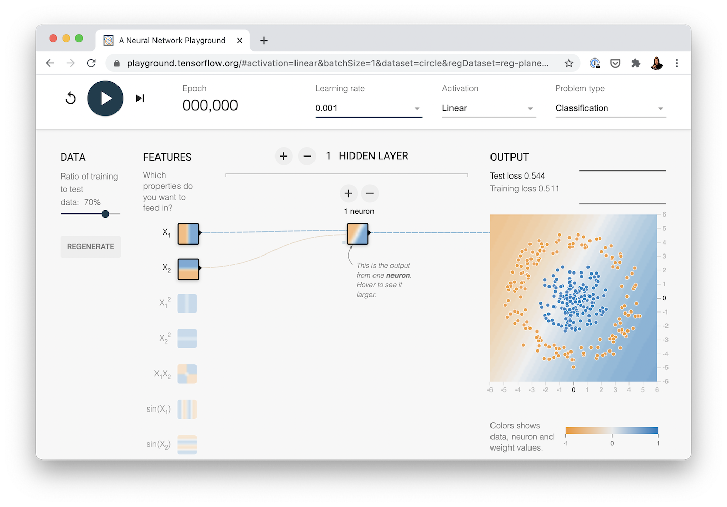The neural network we're going to recreate with TensorFlow code. See it live at TensorFlow Playground.

The main change we'll add to models we've built before is the use of the activation keyword.

In [ ]:

# Set the random seed
tf.random.set_seed(42)

# Create the model
model_4 = tf.keras.Sequential([
  tf.keras.layers.Dense(1, activation=tf.keras.activations.linear), # 1 hidden layer with linear activation
  tf.keras.layers.Dense(1) # output layer
])

# Compile the model
model_4.compile(loss=tf.keras.losses.binary_crossentropy,
                optimizer=tf.keras.optimizers.Adam(lr=0.001), # "lr" is short for "learning rate"
                metrics=["accuracy"])

# Fit the model
history = model_4.fit(X, y, epochs=100)

# Set the random seed tf.random.set_seed(42) # Create the model model_4 = tf.keras.Sequential([ tf.keras.layers.Dense(1, activation=tf.keras.activations.linear), # 1 hidden layer with linear activation tf.keras.layers.Dense(1) # output layer ]) # Compile the model model_4.compile(loss=tf.keras.losses.binary_crossentropy, optimizer=tf.keras.optimizers.Adam(lr=0.001), # "lr" is short for "learning rate" metrics=["accuracy"]) # Fit the model history = model_4.fit(X, y, epochs=100)

/usr/local/lib/python3.7/dist-packages/keras/optimizer_v2/adam.py:105: UserWarning: The `lr` argument is deprecated, use `learning_rate` instead.
  super(Adam, self).__init__(name, **kwargs)

Epoch 1/100
32/32 [==============================] - 1s 2ms/step - loss: 4.2380 - accuracy: 0.5000
Epoch 2/100
32/32 [==============================] - 0s 1ms/step - loss: 4.0223 - accuracy: 0.5000
Epoch 3/100
32/32 [==============================] - 0s 2ms/step - loss: 3.8296 - accuracy: 0.5000
Epoch 4/100
32/32 [==============================] - 0s 2ms/step - loss: 3.7654 - accuracy: 0.5000
Epoch 5/100
32/32 [==============================] - 0s 1ms/step - loss: 3.6464 - accuracy: 0.5000
Epoch 6/100
32/32 [==============================] - 0s 1ms/step - loss: 3.4960 - accuracy: 0.5000
Epoch 7/100
32/32 [==============================] - 0s 2ms/step - loss: 3.3804 - accuracy: 0.5000
Epoch 8/100
32/32 [==============================] - 0s 2ms/step - loss: 3.2279 - accuracy: 0.5000
Epoch 9/100
32/32 [==============================] - 0s 2ms/step - loss: 2.7024 - accuracy: 0.5000
Epoch 10/100
32/32 [==============================] - 0s 2ms/step - loss: 2.4002 - accuracy: 0.5000
Epoch 11/100
32/32 [==============================] - 0s 2ms/step - loss: 2.1984 - accuracy: 0.5000
Epoch 12/100
32/32 [==============================] - 0s 1ms/step - loss: 1.3257 - accuracy: 0.5000
Epoch 13/100
32/32 [==============================] - 0s 2ms/step - loss: 1.0542 - accuracy: 0.5000
Epoch 14/100
32/32 [==============================] - 0s 2ms/step - loss: 1.0261 - accuracy: 0.5000
Epoch 15/100
32/32 [==============================] - 0s 1ms/step - loss: 1.0069 - accuracy: 0.5000
Epoch 16/100
32/32 [==============================] - 0s 2ms/step - loss: 0.9914 - accuracy: 0.5000
Epoch 17/100
32/32 [==============================] - 0s 1ms/step - loss: 0.9776 - accuracy: 0.5000
Epoch 18/100
32/32 [==============================] - 0s 2ms/step - loss: 0.9656 - accuracy: 0.5000
Epoch 19/100
32/32 [==============================] - 0s 2ms/step - loss: 0.9549 - accuracy: 0.5000
Epoch 20/100
32/32 [==============================] - 0s 1ms/step - loss: 0.9448 - accuracy: 0.5000
Epoch 21/100
32/32 [==============================] - 0s 1ms/step - loss: 0.9357 - accuracy: 0.5000
Epoch 22/100
32/32 [==============================] - 0s 1ms/step - loss: 0.9269 - accuracy: 0.5000
Epoch 23/100
32/32 [==============================] - 0s 1ms/step - loss: 0.9190 - accuracy: 0.5000
Epoch 24/100
32/32 [==============================] - 0s 2ms/step - loss: 0.9115 - accuracy: 0.5000
Epoch 25/100
32/32 [==============================] - 0s 2ms/step - loss: 0.9046 - accuracy: 0.5000
Epoch 26/100
32/32 [==============================] - 0s 1ms/step - loss: 0.8976 - accuracy: 0.5000
Epoch 27/100
32/32 [==============================] - 0s 2ms/step - loss: 0.8912 - accuracy: 0.4990
Epoch 28/100
32/32 [==============================] - 0s 1ms/step - loss: 0.8850 - accuracy: 0.4960
Epoch 29/100
32/32 [==============================] - 0s 1ms/step - loss: 0.8790 - accuracy: 0.4950
Epoch 30/100
32/32 [==============================] - 0s 2ms/step - loss: 0.8732 - accuracy: 0.4950
Epoch 31/100
32/32 [==============================] - 0s 1ms/step - loss: 0.8678 - accuracy: 0.4870
Epoch 32/100
32/32 [==============================] - 0s 1ms/step - loss: 0.8623 - accuracy: 0.4790
Epoch 33/100
32/32 [==============================] - 0s 1ms/step - loss: 0.8573 - accuracy: 0.4750
Epoch 34/100
32/32 [==============================] - 0s 1ms/step - loss: 0.8525 - accuracy: 0.4730
Epoch 35/100
32/32 [==============================] - 0s 1ms/step - loss: 0.8477 - accuracy: 0.4650
Epoch 36/100
32/32 [==============================] - 0s 2ms/step - loss: 0.8432 - accuracy: 0.4590
Epoch 37/100
32/32 [==============================] - 0s 2ms/step - loss: 0.8388 - accuracy: 0.4560
Epoch 38/100
32/32 [==============================] - 0s 2ms/step - loss: 0.8347 - accuracy: 0.4470
Epoch 39/100
32/32 [==============================] - 0s 1ms/step - loss: 0.8305 - accuracy: 0.4420
Epoch 40/100
32/32 [==============================] - 0s 1ms/step - loss: 0.8266 - accuracy: 0.4380
Epoch 41/100
32/32 [==============================] - 0s 2ms/step - loss: 0.8227 - accuracy: 0.4340
Epoch 42/100
32/32 [==============================] - 0s 1ms/step - loss: 0.8189 - accuracy: 0.4290
Epoch 43/100
32/32 [==============================] - 0s 2ms/step - loss: 0.8151 - accuracy: 0.4280
Epoch 44/100
32/32 [==============================] - 0s 2ms/step - loss: 0.8116 - accuracy: 0.4280
Epoch 45/100
32/32 [==============================] - 0s 2ms/step - loss: 0.8082 - accuracy: 0.4200
Epoch 46/100
32/32 [==============================] - 0s 1ms/step - loss: 0.8049 - accuracy: 0.4160
Epoch 47/100
32/32 [==============================] - 0s 2ms/step - loss: 0.8018 - accuracy: 0.4150
Epoch 48/100
32/32 [==============================] - 0s 1ms/step - loss: 0.7986 - accuracy: 0.4130
Epoch 49/100
32/32 [==============================] - 0s 1ms/step - loss: 0.7956 - accuracy: 0.4140
Epoch 50/100
32/32 [==============================] - 0s 2ms/step - loss: 0.7926 - accuracy: 0.4170
Epoch 51/100
32/32 [==============================] - 0s 2ms/step - loss: 0.7897 - accuracy: 0.4200
Epoch 52/100
32/32 [==============================] - 0s 1ms/step - loss: 0.7870 - accuracy: 0.4210
Epoch 53/100
32/32 [==============================] - 0s 2ms/step - loss: 0.7843 - accuracy: 0.4280
Epoch 54/100
32/32 [==============================] - 0s 2ms/step - loss: 0.7817 - accuracy: 0.4350
Epoch 55/100
32/32 [==============================] - 0s 1ms/step - loss: 0.7791 - accuracy: 0.4480
Epoch 56/100
32/32 [==============================] - 0s 2ms/step - loss: 0.7766 - accuracy: 0.4510
Epoch 57/100
32/32 [==============================] - 0s 2ms/step - loss: 0.7742 - accuracy: 0.4530
Epoch 58/100
32/32 [==============================] - 0s 1ms/step - loss: 0.7718 - accuracy: 0.4530
Epoch 59/100
32/32 [==============================] - 0s 1ms/step - loss: 0.7696 - accuracy: 0.4550
Epoch 60/100
32/32 [==============================] - 0s 1ms/step - loss: 0.7674 - accuracy: 0.4570
Epoch 61/100
32/32 [==============================] - 0s 1ms/step - loss: 0.7654 - accuracy: 0.4560
Epoch 62/100
32/32 [==============================] - 0s 2ms/step - loss: 0.7634 - accuracy: 0.4600
Epoch 63/100
32/32 [==============================] - 0s 1ms/step - loss: 0.7613 - accuracy: 0.4610
Epoch 64/100
32/32 [==============================] - 0s 1ms/step - loss: 0.7595 - accuracy: 0.4640
Epoch 65/100
32/32 [==============================] - 0s 1ms/step - loss: 0.7577 - accuracy: 0.4590
Epoch 66/100
32/32 [==============================] - 0s 1ms/step - loss: 0.7558 - accuracy: 0.4630
Epoch 67/100
32/32 [==============================] - 0s 2ms/step - loss: 0.7541 - accuracy: 0.4620
Epoch 68/100
32/32 [==============================] - 0s 2ms/step - loss: 0.7524 - accuracy: 0.4640
Epoch 69/100
32/32 [==============================] - 0s 1ms/step - loss: 0.7507 - accuracy: 0.4660
Epoch 70/100
32/32 [==============================] - 0s 2ms/step - loss: 0.7491 - accuracy: 0.4660
Epoch 71/100
32/32 [==============================] - 0s 1ms/step - loss: 0.7475 - accuracy: 0.4680
Epoch 72/100
32/32 [==============================] - 0s 1ms/step - loss: 0.7460 - accuracy: 0.4710
Epoch 73/100
32/32 [==============================] - 0s 1ms/step - loss: 0.7445 - accuracy: 0.4720
Epoch 74/100
32/32 [==============================] - 0s 1ms/step - loss: 0.7430 - accuracy: 0.4740
Epoch 75/100
32/32 [==============================] - 0s 2ms/step - loss: 0.7416 - accuracy: 0.4730
Epoch 76/100
32/32 [==============================] - 0s 1ms/step - loss: 0.7403 - accuracy: 0.4750
Epoch 77/100
32/32 [==============================] - 0s 1ms/step - loss: 0.7390 - accuracy: 0.4730
Epoch 78/100
32/32 [==============================] - 0s 1ms/step - loss: 0.7377 - accuracy: 0.4720
Epoch 79/100
32/32 [==============================] - 0s 1ms/step - loss: 0.7365 - accuracy: 0.4730
Epoch 80/100
32/32 [==============================] - 0s 2ms/step - loss: 0.7353 - accuracy: 0.4760
Epoch 81/100
32/32 [==============================] - 0s 1ms/step - loss: 0.7341 - accuracy: 0.4740
Epoch 82/100
32/32 [==============================] - 0s 1ms/step - loss: 0.7330 - accuracy: 0.4750
Epoch 83/100
32/32 [==============================] - 0s 1ms/step - loss: 0.7320 - accuracy: 0.4790
Epoch 84/100
32/32 [==============================] - 0s 1ms/step - loss: 0.7309 - accuracy: 0.4790
Epoch 85/100
32/32 [==============================] - 0s 1ms/step - loss: 0.7299 - accuracy: 0.4810
Epoch 86/100
32/32 [==============================] - 0s 1ms/step - loss: 0.7290 - accuracy: 0.4820
Epoch 87/100
32/32 [==============================] - 0s 2ms/step - loss: 0.7280 - accuracy: 0.4850
Epoch 88/100
32/32 [==============================] - 0s 1ms/step - loss: 0.7271 - accuracy: 0.4850
Epoch 89/100
32/32 [==============================] - 0s 1ms/step - loss: 0.7263 - accuracy: 0.4870
Epoch 90/100
32/32 [==============================] - 0s 1ms/step - loss: 0.7254 - accuracy: 0.4880
Epoch 91/100
32/32 [==============================] - 0s 1ms/step - loss: 0.7246 - accuracy: 0.4900
Epoch 92/100
32/32 [==============================] - 0s 1ms/step - loss: 0.7238 - accuracy: 0.4890
Epoch 93/100
32/32 [==============================] - 0s 2ms/step - loss: 0.7230 - accuracy: 0.4890
Epoch 94/100
32/32 [==============================] - 0s 2ms/step - loss: 0.7223 - accuracy: 0.4860
Epoch 95/100
32/32 [==============================] - 0s 1ms/step - loss: 0.7215 - accuracy: 0.4860
Epoch 96/100
32/32 [==============================] - 0s 1ms/step - loss: 0.7208 - accuracy: 0.4860
Epoch 97/100
32/32 [==============================] - 0s 1ms/step - loss: 0.7202 - accuracy: 0.4880
Epoch 98/100
32/32 [==============================] - 0s 2ms/step - loss: 0.7195 - accuracy: 0.4870
Epoch 99/100
32/32 [==============================] - 0s 1ms/step - loss: 0.7188 - accuracy: 0.4870
Epoch 100/100
32/32 [==============================] - 0s 1ms/step - loss: 0.7181 - accuracy: 0.4850

Okay, our model performs a little worse than guessing.

Let's remind ourselves what our data looks like.

In [ ]:

# Check out our data
plt.scatter(X[:, 0], X[:, 1], c=y, cmap=plt.cm.RdYlBu);

# Check out our data plt.scatter(X[:, 0], X[:, 1], c=y, cmap=plt.cm.RdYlBu);

And let's see how our model is making predictions on it.

In [ ]:

# Check the deicison boundary (blue is blue class, yellow is the crossover, red is red class)
plot_decision_boundary(model_4, X, y)

# Check the deicison boundary (blue is blue class, yellow is the crossover, red is red class) plot_decision_boundary(model_4, X, y)

doing binary classifcation...

Well, it looks like we're getting a straight (linear) line prediction again.

But our data is non-linear (not a straight line)...

What we're going to have to do is add some non-linearity to our model.

To do so, we'll use the activation parameter in on of our layers.

In [ ]:

# Set random seed
tf.random.set_seed(42)

# Create a model with a non-linear activation
model_5 = tf.keras.Sequential([
  tf.keras.layers.Dense(1, activation=tf.keras.activations.relu), # can also do activation='relu'
  tf.keras.layers.Dense(1) # output layer 
])

# Compile the model
model_5.compile(loss=tf.keras.losses.binary_crossentropy,
              optimizer=tf.keras.optimizers.Adam(),
              metrics=["accuracy"])

# Fit the model
history = model_5.fit(X, y, epochs=100)

# Set random seed tf.random.set_seed(42) # Create a model with a non-linear activation model_5 = tf.keras.Sequential([ tf.keras.layers.Dense(1, activation=tf.keras.activations.relu), # can also do activation='relu' tf.keras.layers.Dense(1) # output layer ]) # Compile the model model_5.compile(loss=tf.keras.losses.binary_crossentropy, optimizer=tf.keras.optimizers.Adam(), metrics=["accuracy"]) # Fit the model history = model_5.fit(X, y, epochs=100)

Epoch 1/100
32/32 [==============================] - 1s 1ms/step - loss: 1.8377 - accuracy: 0.5000
Epoch 2/100
32/32 [==============================] - 0s 1ms/step - loss: 1.4449 - accuracy: 0.5000
Epoch 3/100
32/32 [==============================] - 0s 1ms/step - loss: 1.3410 - accuracy: 0.5000
Epoch 4/100
32/32 [==============================] - 0s 1ms/step - loss: 1.2678 - accuracy: 0.4770
Epoch 5/100
32/32 [==============================] - 0s 1ms/step - loss: 1.2116 - accuracy: 0.4390
Epoch 6/100
32/32 [==============================] - 0s 2ms/step - loss: 1.1664 - accuracy: 0.4180
Epoch 7/100
32/32 [==============================] - 0s 1ms/step - loss: 1.1294 - accuracy: 0.4250
Epoch 8/100
32/32 [==============================] - 0s 1ms/step - loss: 1.0970 - accuracy: 0.4420
Epoch 9/100
32/32 [==============================] - 0s 1ms/step - loss: 1.0670 - accuracy: 0.4540
Epoch 10/100
32/32 [==============================] - 0s 1ms/step - loss: 1.0407 - accuracy: 0.4550
Epoch 11/100
32/32 [==============================] - 0s 1ms/step - loss: 1.0147 - accuracy: 0.4600
Epoch 12/100
32/32 [==============================] - 0s 1ms/step - loss: 0.9872 - accuracy: 0.4630
Epoch 13/100
32/32 [==============================] - 0s 1ms/step - loss: 0.9579 - accuracy: 0.4620
Epoch 14/100
32/32 [==============================] - 0s 1ms/step - loss: 0.9201 - accuracy: 0.4660
Epoch 15/100
32/32 [==============================] - 0s 2ms/step - loss: 0.8514 - accuracy: 0.4660
Epoch 16/100
32/32 [==============================] - 0s 1ms/step - loss: 0.7888 - accuracy: 0.4720
Epoch 17/100
32/32 [==============================] - 0s 1ms/step - loss: 0.7580 - accuracy: 0.4740
Epoch 18/100
32/32 [==============================] - 0s 2ms/step - loss: 0.7392 - accuracy: 0.4760
Epoch 19/100
32/32 [==============================] - 0s 2ms/step - loss: 0.7273 - accuracy: 0.4850
Epoch 20/100
32/32 [==============================] - 0s 1ms/step - loss: 0.7180 - accuracy: 0.4870
Epoch 21/100
32/32 [==============================] - 0s 2ms/step - loss: 0.7121 - accuracy: 0.4880
Epoch 22/100
32/32 [==============================] - 0s 1ms/step - loss: 0.7070 - accuracy: 0.4880
Epoch 23/100
32/32 [==============================] - 0s 2ms/step - loss: 0.7036 - accuracy: 0.4870
Epoch 24/100
32/32 [==============================] - 0s 2ms/step - loss: 0.7011 - accuracy: 0.4900
Epoch 25/100
32/32 [==============================] - 0s 1ms/step - loss: 0.6993 - accuracy: 0.4860
Epoch 26/100
32/32 [==============================] - 0s 2ms/step - loss: 0.6977 - accuracy: 0.4910
Epoch 27/100
32/32 [==============================] - 0s 2ms/step - loss: 0.6970 - accuracy: 0.4950
Epoch 28/100
32/32 [==============================] - 0s 1ms/step - loss: 0.6959 - accuracy: 0.4970
Epoch 29/100
32/32 [==============================] - 0s 1ms/step - loss: 0.6955 - accuracy: 0.4950
Epoch 30/100
32/32 [==============================] - 0s 1ms/step - loss: 0.6949 - accuracy: 0.4970
Epoch 31/100
32/32 [==============================] - 0s 1ms/step - loss: 0.6946 - accuracy: 0.4990
Epoch 32/100
32/32 [==============================] - 0s 1ms/step - loss: 0.6943 - accuracy: 0.4910
Epoch 33/100
32/32 [==============================] - 0s 2ms/step - loss: 0.6940 - accuracy: 0.5000
Epoch 34/100
32/32 [==============================] - 0s 1ms/step - loss: 0.6939 - accuracy: 0.4910
Epoch 35/100
32/32 [==============================] - 0s 1ms/step - loss: 0.6937 - accuracy: 0.4940
Epoch 36/100
32/32 [==============================] - 0s 1ms/step - loss: 0.6935 - accuracy: 0.4930
Epoch 37/100
32/32 [==============================] - 0s 2ms/step - loss: 0.6934 - accuracy: 0.4950
Epoch 38/100
32/32 [==============================] - 0s 2ms/step - loss: 0.6935 - accuracy: 0.4900
Epoch 39/100
32/32 [==============================] - 0s 1ms/step - loss: 0.6934 - accuracy: 0.4840
Epoch 40/100
32/32 [==============================] - 0s 1ms/step - loss: 0.6935 - accuracy: 0.5000
Epoch 41/100
32/32 [==============================] - 0s 2ms/step - loss: 0.6936 - accuracy: 0.5060
Epoch 42/100
32/32 [==============================] - 0s 2ms/step - loss: 0.6935 - accuracy: 0.4800
Epoch 43/100
32/32 [==============================] - 0s 1ms/step - loss: 0.6933 - accuracy: 0.5050
Epoch 44/100
32/32 [==============================] - 0s 1ms/step - loss: 0.6936 - accuracy: 0.4810
Epoch 45/100
32/32 [==============================] - 0s 2ms/step - loss: 0.6933 - accuracy: 0.4550
Epoch 46/100
32/32 [==============================] - 0s 1ms/step - loss: 0.6932 - accuracy: 0.4920
Epoch 47/100
32/32 [==============================] - 0s 1ms/step - loss: 0.6935 - accuracy: 0.4870
Epoch 48/100
32/32 [==============================] - 0s 2ms/step - loss: 0.6934 - accuracy: 0.5100
Epoch 49/100
32/32 [==============================] - 0s 1ms/step - loss: 0.6934 - accuracy: 0.4770
Epoch 50/100
32/32 [==============================] - 0s 1ms/step - loss: 0.6934 - accuracy: 0.5000
Epoch 51/100
32/32 [==============================] - 0s 1ms/step - loss: 0.6933 - accuracy: 0.4760
Epoch 52/100
32/32 [==============================] - 0s 1ms/step - loss: 0.6934 - accuracy: 0.5010
Epoch 53/100
32/32 [==============================] - 0s 1ms/step - loss: 0.6935 - accuracy: 0.4880
Epoch 54/100
32/32 [==============================] - 0s 1ms/step - loss: 0.6933 - accuracy: 0.5530
Epoch 55/100
32/32 [==============================] - 0s 2ms/step - loss: 0.6935 - accuracy: 0.5060
Epoch 56/100
32/32 [==============================] - 0s 2ms/step - loss: 0.6935 - accuracy: 0.5200
Epoch 57/100
32/32 [==============================] - 0s 2ms/step - loss: 0.6933 - accuracy: 0.4910
Epoch 58/100
32/32 [==============================] - 0s 1ms/step - loss: 0.6934 - accuracy: 0.4990
Epoch 59/100
32/32 [==============================] - 0s 2ms/step - loss: 0.6938 - accuracy: 0.5000
Epoch 60/100
32/32 [==============================] - 0s 2ms/step - loss: 0.6934 - accuracy: 0.5000
Epoch 61/100
32/32 [==============================] - 0s 1ms/step - loss: 0.6935 - accuracy: 0.4900
Epoch 62/100
32/32 [==============================] - 0s 1ms/step - loss: 0.6934 - accuracy: 0.4820
Epoch 63/100
32/32 [==============================] - 0s 1ms/step - loss: 0.6933 - accuracy: 0.4700
Epoch 64/100
32/32 [==============================] - 0s 2ms/step - loss: 0.6934 - accuracy: 0.4820
Epoch 65/100
32/32 [==============================] - 0s 2ms/step - loss: 0.6934 - accuracy: 0.4620
Epoch 66/100
32/32 [==============================] - 0s 2ms/step - loss: 0.6934 - accuracy: 0.4760
Epoch 67/100
32/32 [==============================] - 0s 1ms/step - loss: 0.6934 - accuracy: 0.4830
Epoch 68/100
32/32 [==============================] - 0s 1ms/step - loss: 0.6933 - accuracy: 0.4680
Epoch 69/100
32/32 [==============================] - 0s 1ms/step - loss: 0.6933 - accuracy: 0.5010
Epoch 70/100
32/32 [==============================] - 0s 2ms/step - loss: 0.6934 - accuracy: 0.4970
Epoch 71/100
32/32 [==============================] - 0s 1ms/step - loss: 0.6933 - accuracy: 0.4680
Epoch 72/100
32/32 [==============================] - 0s 2ms/step - loss: 0.6934 - accuracy: 0.5070
Epoch 73/100
32/32 [==============================] - 0s 2ms/step - loss: 0.6934 - accuracy: 0.5320
Epoch 74/100
32/32 [==============================] - 0s 2ms/step - loss: 0.6933 - accuracy: 0.5290
Epoch 75/100
32/32 [==============================] - 0s 1ms/step - loss: 0.6935 - accuracy: 0.5000
Epoch 76/100
32/32 [==============================] - 0s 2ms/step - loss: 0.6935 - accuracy: 0.4730
Epoch 77/100
32/32 [==============================] - 0s 2ms/step - loss: 0.6935 - accuracy: 0.4870
Epoch 78/100
32/32 [==============================] - 0s 2ms/step - loss: 0.6934 - accuracy: 0.4830
Epoch 79/100
32/32 [==============================] - 0s 1ms/step - loss: 0.6935 - accuracy: 0.4640
Epoch 80/100
32/32 [==============================] - 0s 1ms/step - loss: 0.6933 - accuracy: 0.5040
Epoch 81/100
32/32 [==============================] - 0s 2ms/step - loss: 0.6936 - accuracy: 0.5000
Epoch 82/100
32/32 [==============================] - 0s 1ms/step - loss: 0.6935 - accuracy: 0.5020
Epoch 83/100
32/32 [==============================] - 0s 1ms/step - loss: 0.6936 - accuracy: 0.4840
Epoch 84/100
32/32 [==============================] - 0s 2ms/step - loss: 0.6932 - accuracy: 0.5070
Epoch 85/100
32/32 [==============================] - 0s 1ms/step - loss: 0.6933 - accuracy: 0.5000
Epoch 86/100
32/32 [==============================] - 0s 1ms/step - loss: 0.6935 - accuracy: 0.5000
Epoch 87/100
32/32 [==============================] - 0s 2ms/step - loss: 0.6933 - accuracy: 0.5000
Epoch 88/100
32/32 [==============================] - 0s 1ms/step - loss: 0.6933 - accuracy: 0.4680
Epoch 89/100
32/32 [==============================] - 0s 1ms/step - loss: 0.6934 - accuracy: 0.4590
Epoch 90/100
32/32 [==============================] - 0s 2ms/step - loss: 0.6937 - accuracy: 0.4980
Epoch 91/100
32/32 [==============================] - 0s 2ms/step - loss: 0.6933 - accuracy: 0.4910
Epoch 92/100
32/32 [==============================] - 0s 2ms/step - loss: 0.6935 - accuracy: 0.4850
Epoch 93/100
32/32 [==============================] - 0s 2ms/step - loss: 0.6938 - accuracy: 0.4970
Epoch 94/100
32/32 [==============================] - 0s 2ms/step - loss: 0.6934 - accuracy: 0.4710
Epoch 95/100
32/32 [==============================] - 0s 1ms/step - loss: 0.6934 - accuracy: 0.4720
Epoch 96/100
32/32 [==============================] - 0s 2ms/step - loss: 0.6934 - accuracy: 0.4880
Epoch 97/100
32/32 [==============================] - 0s 1ms/step - loss: 0.6934 - accuracy: 0.4510
Epoch 98/100
32/32 [==============================] - 0s 2ms/step - loss: 0.6934 - accuracy: 0.4640
Epoch 99/100
32/32 [==============================] - 0s 1ms/step - loss: 0.6935 - accuracy: 0.4940
Epoch 100/100
32/32 [==============================] - 0s 1ms/step - loss: 0.6936 - accuracy: 0.5180

Hmm... still not learning...

What we if increased the number of neurons and layers?

Say, 2 hidden layers, with ReLU, pronounced "rel-u", (short for rectified linear unit), activation on the first one, and 4 neurons each?

To see this network in action, check out the TensorFlow Playground demo.

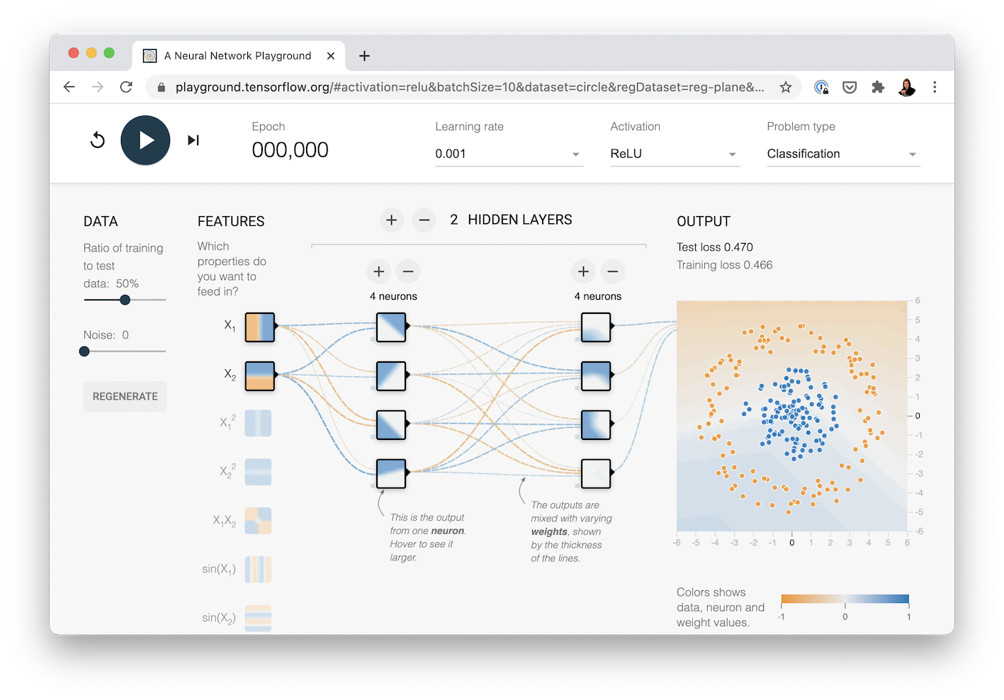The neural network we're going to recreate with TensorFlow code. See it live at TensorFlow Playground.

Let's try.

In [ ]:

# Set random seed
tf.random.set_seed(42)

# Create a model
model_6 = tf.keras.Sequential([
  tf.keras.layers.Dense(4, activation=tf.keras.activations.relu), # hidden layer 1, 4 neurons, ReLU activation
  tf.keras.layers.Dense(4, activation=tf.keras.activations.relu), # hidden layer 2, 4 neurons, ReLU activation
  tf.keras.layers.Dense(1) # ouput layer
])

# Compile the model
model_6.compile(loss=tf.keras.losses.binary_crossentropy,
                optimizer=tf.keras.optimizers.Adam(lr=0.001), # Adam's default learning rate is 0.001
                metrics=['accuracy'])

# Fit the model
history = model_6.fit(X, y, epochs=100)

# Set random seed tf.random.set_seed(42) # Create a model model_6 = tf.keras.Sequential([ tf.keras.layers.Dense(4, activation=tf.keras.activations.relu), # hidden layer 1, 4 neurons, ReLU activation tf.keras.layers.Dense(4, activation=tf.keras.activations.relu), # hidden layer 2, 4 neurons, ReLU activation tf.keras.layers.Dense(1) # ouput layer ]) # Compile the model model_6.compile(loss=tf.keras.losses.binary_crossentropy, optimizer=tf.keras.optimizers.Adam(lr=0.001), # Adam's default learning rate is 0.001 metrics=['accuracy']) # Fit the model history = model_6.fit(X, y, epochs=100)

/usr/local/lib/python3.7/dist-packages/keras/optimizer_v2/adam.py:105: UserWarning: The `lr` argument is deprecated, use `learning_rate` instead.
  super(Adam, self).__init__(name, **kwargs)

Epoch 1/100
32/32 [==============================] - 1s 2ms/step - loss: 7.7125 - accuracy: 0.5000
Epoch 2/100
32/32 [==============================] - 0s 2ms/step - loss: 7.7125 - accuracy: 0.5000
Epoch 3/100
32/32 [==============================] - 0s 1ms/step - loss: 7.7125 - accuracy: 0.5000
Epoch 4/100
32/32 [==============================] - 0s 2ms/step - loss: 7.7125 - accuracy: 0.5000
Epoch 5/100
32/32 [==============================] - 0s 2ms/step - loss: 7.7125 - accuracy: 0.5000
Epoch 6/100
32/32 [==============================] - 0s 2ms/step - loss: 7.7125 - accuracy: 0.5000
Epoch 7/100
32/32 [==============================] - 0s 1ms/step - loss: 7.7125 - accuracy: 0.5000
Epoch 8/100
32/32 [==============================] - 0s 2ms/step - loss: 7.7125 - accuracy: 0.5000
Epoch 9/100
32/32 [==============================] - 0s 2ms/step - loss: 7.7125 - accuracy: 0.5000
Epoch 10/100
32/32 [==============================] - 0s 2ms/step - loss: 7.7125 - accuracy: 0.5000
Epoch 11/100
32/32 [==============================] - 0s 2ms/step - loss: 7.7125 - accuracy: 0.5000
Epoch 12/100
32/32 [==============================] - 0s 2ms/step - loss: 7.7125 - accuracy: 0.5000
Epoch 13/100
32/32 [==============================] - 0s 2ms/step - loss: 7.7125 - accuracy: 0.5000
Epoch 14/100
32/32 [==============================] - 0s 2ms/step - loss: 7.7125 - accuracy: 0.5000
Epoch 15/100
32/32 [==============================] - 0s 2ms/step - loss: 7.7125 - accuracy: 0.5000
Epoch 16/100
32/32 [==============================] - 0s 2ms/step - loss: 7.7125 - accuracy: 0.5000
Epoch 17/100
32/32 [==============================] - 0s 1ms/step - loss: 7.7125 - accuracy: 0.5000
Epoch 18/100
32/32 [==============================] - 0s 1ms/step - loss: 7.7125 - accuracy: 0.5000
Epoch 19/100
32/32 [==============================] - 0s 1ms/step - loss: 7.7125 - accuracy: 0.5000
Epoch 20/100
32/32 [==============================] - 0s 2ms/step - loss: 7.7125 - accuracy: 0.5000
Epoch 21/100
32/32 [==============================] - 0s 2ms/step - loss: 7.7125 - accuracy: 0.5000
Epoch 22/100
32/32 [==============================] - 0s 1ms/step - loss: 7.7125 - accuracy: 0.5000
Epoch 23/100
32/32 [==============================] - 0s 1ms/step - loss: 7.7125 - accuracy: 0.5000
Epoch 24/100
32/32 [==============================] - 0s 2ms/step - loss: 7.7125 - accuracy: 0.5000
Epoch 25/100
32/32 [==============================] - 0s 1ms/step - loss: 7.7125 - accuracy: 0.5000
Epoch 26/100
32/32 [==============================] - 0s 1ms/step - loss: 7.7125 - accuracy: 0.5000
Epoch 27/100
32/32 [==============================] - 0s 2ms/step - loss: 7.7125 - accuracy: 0.5000
Epoch 28/100
32/32 [==============================] - 0s 2ms/step - loss: 7.7125 - accuracy: 0.5000
Epoch 29/100
32/32 [==============================] - 0s 1ms/step - loss: 7.7125 - accuracy: 0.5000
Epoch 30/100
32/32 [==============================] - 0s 2ms/step - loss: 7.7125 - accuracy: 0.5000
Epoch 31/100
32/32 [==============================] - 0s 2ms/step - loss: 7.7125 - accuracy: 0.5000
Epoch 32/100
32/32 [==============================] - 0s 2ms/step - loss: 7.7125 - accuracy: 0.5000
Epoch 33/100
32/32 [==============================] - 0s 2ms/step - loss: 7.7125 - accuracy: 0.5000
Epoch 34/100
32/32 [==============================] - 0s 2ms/step - loss: 7.7125 - accuracy: 0.5000
Epoch 35/100
32/32 [==============================] - 0s 2ms/step - loss: 7.7125 - accuracy: 0.5000
Epoch 36/100
32/32 [==============================] - 0s 2ms/step - loss: 7.7125 - accuracy: 0.5000
Epoch 37/100
32/32 [==============================] - 0s 1ms/step - loss: 7.7125 - accuracy: 0.5000
Epoch 38/100
32/32 [==============================] - 0s 1ms/step - loss: 7.7125 - accuracy: 0.5000
Epoch 39/100
32/32 [==============================] - 0s 2ms/step - loss: 7.7125 - accuracy: 0.5000
Epoch 40/100
32/32 [==============================] - 0s 2ms/step - loss: 7.7125 - accuracy: 0.5000
Epoch 41/100
32/32 [==============================] - 0s 2ms/step - loss: 7.7125 - accuracy: 0.5000
Epoch 42/100
32/32 [==============================] - 0s 2ms/step - loss: 7.7125 - accuracy: 0.5000
Epoch 43/100
32/32 [==============================] - 0s 2ms/step - loss: 7.7125 - accuracy: 0.5000
Epoch 44/100
32/32 [==============================] - 0s 1ms/step - loss: 7.7125 - accuracy: 0.5000
Epoch 45/100
32/32 [==============================] - 0s 2ms/step - loss: 7.7125 - accuracy: 0.5000
Epoch 46/100
32/32 [==============================] - 0s 2ms/step - loss: 7.7125 - accuracy: 0.5000
Epoch 47/100
32/32 [==============================] - 0s 2ms/step - loss: 7.7125 - accuracy: 0.5000
Epoch 48/100
32/32 [==============================] - 0s 1ms/step - loss: 7.7125 - accuracy: 0.5000
Epoch 49/100
32/32 [==============================] - 0s 1ms/step - loss: 7.7125 - accuracy: 0.5000
Epoch 50/100
32/32 [==============================] - 0s 1ms/step - loss: 7.7125 - accuracy: 0.5000
Epoch 51/100
32/32 [==============================] - 0s 1ms/step - loss: 7.7125 - accuracy: 0.5000
Epoch 52/100
32/32 [==============================] - 0s 1ms/step - loss: 7.7125 - accuracy: 0.5000
Epoch 53/100
32/32 [==============================] - 0s 2ms/step - loss: 7.7125 - accuracy: 0.5000
Epoch 54/100
32/32 [==============================] - 0s 1ms/step - loss: 7.7125 - accuracy: 0.5000
Epoch 55/100
32/32 [==============================] - 0s 2ms/step - loss: 7.7125 - accuracy: 0.5000
Epoch 56/100
32/32 [==============================] - 0s 1ms/step - loss: 7.7125 - accuracy: 0.5000
Epoch 57/100
32/32 [==============================] - 0s 1ms/step - loss: 7.7125 - accuracy: 0.5000
Epoch 58/100
32/32 [==============================] - 0s 2ms/step - loss: 7.7125 - accuracy: 0.5000
Epoch 59/100
32/32 [==============================] - 0s 2ms/step - loss: 7.7125 - accuracy: 0.5000
Epoch 60/100
32/32 [==============================] - 0s 2ms/step - loss: 7.7125 - accuracy: 0.5000
Epoch 61/100
32/32 [==============================] - 0s 2ms/step - loss: 7.7125 - accuracy: 0.5000
Epoch 62/100
32/32 [==============================] - 0s 2ms/step - loss: 7.7125 - accuracy: 0.5000
Epoch 63/100
32/32 [==============================] - 0s 2ms/step - loss: 7.7125 - accuracy: 0.5000
Epoch 64/100
32/32 [==============================] - 0s 2ms/step - loss: 7.7125 - accuracy: 0.5000
Epoch 65/100
32/32 [==============================] - 0s 2ms/step - loss: 7.7125 - accuracy: 0.5000
Epoch 66/100
32/32 [==============================] - 0s 1ms/step - loss: 7.7125 - accuracy: 0.5000
Epoch 67/100
32/32 [==============================] - 0s 1ms/step - loss: 7.7125 - accuracy: 0.5000
Epoch 68/100
32/32 [==============================] - 0s 1ms/step - loss: 7.7125 - accuracy: 0.5000
Epoch 69/100
32/32 [==============================] - 0s 1ms/step - loss: 7.7125 - accuracy: 0.5000
Epoch 70/100
32/32 [==============================] - 0s 2ms/step - loss: 7.7125 - accuracy: 0.5000
Epoch 71/100
32/32 [==============================] - 0s 2ms/step - loss: 7.7125 - accuracy: 0.5000
Epoch 72/100
32/32 [==============================] - 0s 2ms/step - loss: 7.7125 - accuracy: 0.5000
Epoch 73/100
32/32 [==============================] - 0s 1ms/step - loss: 7.7125 - accuracy: 0.5000
Epoch 74/100
32/32 [==============================] - 0s 1ms/step - loss: 7.7125 - accuracy: 0.5000
Epoch 75/100
32/32 [==============================] - 0s 2ms/step - loss: 7.7125 - accuracy: 0.5000
Epoch 76/100
32/32 [==============================] - 0s 1ms/step - loss: 7.7125 - accuracy: 0.5000
Epoch 77/100
32/32 [==============================] - 0s 2ms/step - loss: 7.7125 - accuracy: 0.5000
Epoch 78/100
32/32 [==============================] - 0s 2ms/step - loss: 7.7125 - accuracy: 0.5000
Epoch 79/100
32/32 [==============================] - 0s 1ms/step - loss: 7.7125 - accuracy: 0.5000
Epoch 80/100
32/32 [==============================] - 0s 2ms/step - loss: 7.7125 - accuracy: 0.5000
Epoch 81/100
32/32 [==============================] - 0s 1ms/step - loss: 7.7125 - accuracy: 0.5000
Epoch 82/100
32/32 [==============================] - 0s 2ms/step - loss: 7.7125 - accuracy: 0.5000
Epoch 83/100
32/32 [==============================] - 0s 1ms/step - loss: 7.7125 - accuracy: 0.5000
Epoch 84/100
32/32 [==============================] - 0s 1ms/step - loss: 7.7125 - accuracy: 0.5000
Epoch 85/100
32/32 [==============================] - 0s 2ms/step - loss: 7.7125 - accuracy: 0.5000
Epoch 86/100
32/32 [==============================] - 0s 2ms/step - loss: 7.7125 - accuracy: 0.5000
Epoch 87/100
32/32 [==============================] - 0s 2ms/step - loss: 7.7125 - accuracy: 0.5000
Epoch 88/100
32/32 [==============================] - 0s 2ms/step - loss: 7.7125 - accuracy: 0.5000
Epoch 89/100
32/32 [==============================] - 0s 1ms/step - loss: 7.7125 - accuracy: 0.5000
Epoch 90/100
32/32 [==============================] - 0s 2ms/step - loss: 7.7125 - accuracy: 0.5000
Epoch 91/100
32/32 [==============================] - 0s 1ms/step - loss: 7.7125 - accuracy: 0.5000
Epoch 92/100
32/32 [==============================] - 0s 1ms/step - loss: 7.7125 - accuracy: 0.5000
Epoch 93/100
32/32 [==============================] - 0s 2ms/step - loss: 7.7125 - accuracy: 0.5000
Epoch 94/100
32/32 [==============================] - 0s 2ms/step - loss: 7.7125 - accuracy: 0.5000
Epoch 95/100
32/32 [==============================] - 0s 3ms/step - loss: 7.7125 - accuracy: 0.5000
Epoch 96/100
32/32 [==============================] - 0s 2ms/step - loss: 7.7125 - accuracy: 0.5000
Epoch 97/100
32/32 [==============================] - 0s 2ms/step - loss: 7.7125 - accuracy: 0.5000
Epoch 98/100
32/32 [==============================] - 0s 2ms/step - loss: 7.7125 - accuracy: 0.5000
Epoch 99/100
32/32 [==============================] - 0s 2ms/step - loss: 7.7125 - accuracy: 0.5000
Epoch 100/100
32/32 [==============================] - 0s 2ms/step - loss: 7.7125 - accuracy: 0.5000

In [ ]:

# Evaluate the model
model_6.evaluate(X, y)

# Evaluate the model model_6.evaluate(X, y)

32/32 [==============================] - 0s 1ms/step - loss: 7.7125 - accuracy: 0.5000

Out[ ]:

[7.712474346160889, 0.5]

We're still hitting 50% accuracy, our model is still practically as good as guessing.

How do the predictions look?

In [ ]:

# Check out the predictions using 2 hidden layers
plot_decision_boundary(model_6, X, y)

# Check out the predictions using 2 hidden layers plot_decision_boundary(model_6, X, y)

doing binary classifcation...

What gives?

It seems like our model is the same as the one in the TensorFlow Playground but model it's still drawing straight lines...

Ideally, the yellow lines go on the inside of the red circle and the blue circle.

Okay, okay, let's model this circle once and for all.

One more model (I promise... actually, I'm going to have to break that promise... we'll be building plenty more models).

This time we'll change the activation function on our output layer too. Remember the architecture of a classification model? For binary classification, the output layer activation is usually the Sigmoid activation function.

In [ ]:

# Set random seed
tf.random.set_seed(42)

# Create a model
model_7 = tf.keras.Sequential([
  tf.keras.layers.Dense(4, activation=tf.keras.activations.relu), # hidden layer 1, ReLU activation
  tf.keras.layers.Dense(4, activation=tf.keras.activations.relu), # hidden layer 2, ReLU activation
  tf.keras.layers.Dense(1, activation=tf.keras.activations.sigmoid) # ouput layer, sigmoid activation
])

# Compile the model
model_7.compile(loss=tf.keras.losses.binary_crossentropy,
                optimizer=tf.keras.optimizers.Adam(),
                metrics=['accuracy'])

# Fit the model
history = model_7.fit(X, y, epochs=100, verbose=0)

# Set random seed tf.random.set_seed(42) # Create a model model_7 = tf.keras.Sequential([ tf.keras.layers.Dense(4, activation=tf.keras.activations.relu), # hidden layer 1, ReLU activation tf.keras.layers.Dense(4, activation=tf.keras.activations.relu), # hidden layer 2, ReLU activation tf.keras.layers.Dense(1, activation=tf.keras.activations.sigmoid) # ouput layer, sigmoid activation ]) # Compile the model model_7.compile(loss=tf.keras.losses.binary_crossentropy, optimizer=tf.keras.optimizers.Adam(), metrics=['accuracy']) # Fit the model history = model_7.fit(X, y, epochs=100, verbose=0)

In [ ]:

# Evaluate our model
model_7.evaluate(X, y)

# Evaluate our model model_7.evaluate(X, y)

32/32 [==============================] - 0s 1ms/step - loss: 0.2948 - accuracy: 0.9910

Out[ ]:

[0.2948004901409149, 0.9909999966621399]

Woah! It looks like our model is getting some incredible results, let's check them out.

In [ ]:

# View the predictions of the model with relu and sigmoid activations
plot_decision_boundary(model_7, X, y)

# View the predictions of the model with relu and sigmoid activations plot_decision_boundary(model_7, X, y)

doing binary classifcation...

Nice! It looks like our model is almost perfectly (apart from a few examples) separating the two circles.

🤔 Question: What's wrong with the predictions we've made? Are we really evaluating our model correctly here? Hint: what data did the model learn on and what did we predict on?

Before we answer that, it's important to recognize what we've just covered.

🔑 Note: The combination of linear (straight lines) and non-linear (non-straight lines) functions is one of the key fundamentals of neural networks.

Think of it like this:

If I gave you an unlimited amount of straight lines and non-straight lines, what kind of patterns could you draw?

That's essentially what neural networks do to find patterns in data.

Now you might be thinking, "but I haven't seen a linear function or a non-linear function before..."

Oh but you have.

We've been using them the whole time.

They're what power the layers in the models we just built.

To get some intuition about the activation functions we've just used, let's create them and then try them on some toy data.

In [ ]:

# Create a toy tensor (similar to the data we pass into our model)
A = tf.cast(tf.range(-10, 10), tf.float32)
A

# Create a toy tensor (similar to the data we pass into our model) A = tf.cast(tf.range(-10, 10), tf.float32) A

Out[ ]:

<tf.Tensor: shape=(20,), dtype=float32, numpy=
array([-10.,  -9.,  -8.,  -7.,  -6.,  -5.,  -4.,  -3.,  -2.,  -1.,   0.,
         1.,   2.,   3.,   4.,   5.,   6.,   7.,   8.,   9.],
      dtype=float32)>

How does this look?

In [ ]:

# Visualize our toy tensor
plt.plot(A);

# Visualize our toy tensor plt.plot(A);

A straight (linear) line!

Nice, now let's recreate the sigmoid function and see what it does to our data. You can also find a pre-built sigmoid function at tf.keras.activations.sigmoid.

In [ ]:

# Sigmoid - https://www.tensorflow.org/api_docs/python/tf/keras/activations/sigmoid
def sigmoid(x):
  return 1 / (1 + tf.exp(-x))

# Use the sigmoid function on our tensor
sigmoid(A)

# Sigmoid - https://www.tensorflow.org/api_docs/python/tf/keras/activations/sigmoid def sigmoid(x): return 1 / (1 + tf.exp(-x)) # Use the sigmoid function on our tensor sigmoid(A)

Out[ ]:

<tf.Tensor: shape=(20,), dtype=float32, numpy=
array([4.5397872e-05, 1.2339458e-04, 3.3535014e-04, 9.1105117e-04,
       2.4726233e-03, 6.6928510e-03, 1.7986210e-02, 4.7425874e-02,
       1.1920292e-01, 2.6894143e-01, 5.0000000e-01, 7.3105860e-01,
       8.8079703e-01, 9.5257413e-01, 9.8201376e-01, 9.9330717e-01,
       9.9752742e-01, 9.9908900e-01, 9.9966466e-01, 9.9987662e-01],
      dtype=float32)>

And how does it look?

In [ ]:

# Plot sigmoid modified tensor
plt.plot(sigmoid(A));

# Plot sigmoid modified tensor plt.plot(sigmoid(A));

A non-straight (non-linear) line!

Okay, how about the ReLU function (ReLU turns all negatives to 0 and positive numbers stay the same)?

In [ ]:

# ReLU - https://www.tensorflow.org/api_docs/python/tf/keras/activations/relu
def relu(x):
  return tf.maximum(0, x)

# Pass toy tensor through ReLU function
relu(A)

# ReLU - https://www.tensorflow.org/api_docs/python/tf/keras/activations/relu def relu(x): return tf.maximum(0, x) # Pass toy tensor through ReLU function relu(A)

Out[ ]:

<tf.Tensor: shape=(20,), dtype=float32, numpy=
array([0., 0., 0., 0., 0., 0., 0., 0., 0., 0., 0., 1., 2., 3., 4., 5., 6.,
       7., 8., 9.], dtype=float32)>

How does the ReLU-modified tensor look?

In [ ]:

# Plot ReLU-modified tensor
plt.plot(relu(A));

# Plot ReLU-modified tensor plt.plot(relu(A));

Another non-straight line!

Well, how about TensorFlow's linear activation function?

In [ ]:

# Linear - https://www.tensorflow.org/api_docs/python/tf/keras/activations/linear (returns input non-modified...)
tf.keras.activations.linear(A)

# Linear - https://www.tensorflow.org/api_docs/python/tf/keras/activations/linear (returns input non-modified...) tf.keras.activations.linear(A)

Out[ ]:

<tf.Tensor: shape=(20,), dtype=float32, numpy=
array([-10.,  -9.,  -8.,  -7.,  -6.,  -5.,  -4.,  -3.,  -2.,  -1.,   0.,
         1.,   2.,   3.,   4.,   5.,   6.,   7.,   8.,   9.],
      dtype=float32)>

Hmm, it looks like our inputs are unmodified...

In [ ]:

# Does the linear activation change anything?
A == tf.keras.activations.linear(A)

# Does the linear activation change anything? A == tf.keras.activations.linear(A)

Out[ ]:

<tf.Tensor: shape=(20,), dtype=bool, numpy=
array([ True,  True,  True,  True,  True,  True,  True,  True,  True,
        True,  True,  True,  True,  True,  True,  True,  True,  True,
        True,  True])>

Okay, so it makes sense now the model doesn't really learn anything when using only linear activation functions, because the linear activation function doesn't change our input data in anyway.

Where as, with our non-linear functions, our data gets manipulated. A neural network uses these kind of transformations at a large scale to figure draw patterns between its inputs and outputs.

Now rather than dive into the guts of neural networks, we're going to keep coding applying what we've learned to different problems but if you want a more in-depth look at what's going on behind the scenes, check out the Extra Curriculum section below.

📖 Resource: For more on activation functions, check out the machine learning cheatsheet page on them.

Evaluating and improving our classification model¶

If you answered the question above, you might've picked up what we've been doing wrong.

We've been evaluating our model on the same data it was trained on.

A better approach would be to split our data into training, validation (optional) and test sets.

Once we've done that, we'll train our model on the training set (let it find patterns in the data) and then see how well it learned the patterns by using it to predict values on the test set.

Let's do it.

In [ ]:

# How many examples are in the whole dataset?
len(X)

# How many examples are in the whole dataset? len(X)

Out[ ]:

1000

In [ ]:

# Split data into train and test sets
X_train, y_train = X[:800], y[:800] # 80% of the data for the training set
X_test, y_test = X[800:], y[800:] # 20% of the data for the test set

# Check the shapes of the data
X_train.shape, X_test.shape # 800 examples in the training set, 200 examples in the test set

# Split data into train and test sets X_train, y_train = X[:800], y[:800] # 80% of the data for the training set X_test, y_test = X[800:], y[800:] # 20% of the data for the test set # Check the shapes of the data X_train.shape, X_test.shape # 800 examples in the training set, 200 examples in the test set

Out[ ]:

((800, 2), (200, 2))

Great, now we've got training and test sets, let's model the training data and evaluate what our model has learned on the test set.

In [ ]:

# Set random seed
tf.random.set_seed(42)

# Create the model (same as model_7)
model_8 = tf.keras.Sequential([
  tf.keras.layers.Dense(4, activation="relu"), # hidden layer 1, using "relu" for activation (same as tf.keras.activations.relu)
  tf.keras.layers.Dense(4, activation="relu"),
  tf.keras.layers.Dense(1, activation="sigmoid") # output layer, using 'sigmoid' for the output
])

# Compile the model
model_8.compile(loss=tf.keras.losses.binary_crossentropy,
                optimizer=tf.keras.optimizers.Adam(lr=0.01), # increase learning rate from 0.001 to 0.01 for faster learning
                metrics=['accuracy'])

# Fit the model
history = model_8.fit(X_train, y_train, epochs=25)

# Set random seed tf.random.set_seed(42) # Create the model (same as model_7) model_8 = tf.keras.Sequential([ tf.keras.layers.Dense(4, activation="relu"), # hidden layer 1, using "relu" for activation (same as tf.keras.activations.relu) tf.keras.layers.Dense(4, activation="relu"), tf.keras.layers.Dense(1, activation="sigmoid") # output layer, using 'sigmoid' for the output ]) # Compile the model model_8.compile(loss=tf.keras.losses.binary_crossentropy, optimizer=tf.keras.optimizers.Adam(lr=0.01), # increase learning rate from 0.001 to 0.01 for faster learning metrics=['accuracy']) # Fit the model history = model_8.fit(X_train, y_train, epochs=25)

/usr/local/lib/python3.7/dist-packages/keras/optimizer_v2/adam.py:105: UserWarning: The `lr` argument is deprecated, use `learning_rate` instead.
  super(Adam, self).__init__(name, **kwargs)

Epoch 1/25
25/25 [==============================] - 0s 2ms/step - loss: 0.6847 - accuracy: 0.5425
Epoch 2/25
25/25 [==============================] - 0s 1ms/step - loss: 0.6777 - accuracy: 0.5525
Epoch 3/25
25/25 [==============================] - 0s 2ms/step - loss: 0.6736 - accuracy: 0.5512
Epoch 4/25
25/25 [==============================] - 0s 2ms/step - loss: 0.6681 - accuracy: 0.5775
Epoch 5/25
25/25 [==============================] - 0s 1ms/step - loss: 0.6633 - accuracy: 0.5850
Epoch 6/25
25/25 [==============================] - 0s 2ms/step - loss: 0.6546 - accuracy: 0.5838
Epoch 7/25
25/25 [==============================] - 0s 1ms/step - loss: 0.6413 - accuracy: 0.6750
Epoch 8/25
25/25 [==============================] - 0s 2ms/step - loss: 0.6264 - accuracy: 0.7013
Epoch 9/25
25/25 [==============================] - 0s 1ms/step - loss: 0.6038 - accuracy: 0.7487
Epoch 10/25
25/25 [==============================] - 0s 2ms/step - loss: 0.5714 - accuracy: 0.7738
Epoch 11/25
25/25 [==============================] - 0s 2ms/step - loss: 0.5404 - accuracy: 0.7650
Epoch 12/25
25/25 [==============================] - 0s 2ms/step - loss: 0.5015 - accuracy: 0.7837
Epoch 13/25
25/25 [==============================] - 0s 2ms/step - loss: 0.4683 - accuracy: 0.7975
Epoch 14/25
25/25 [==============================] - 0s 2ms/step - loss: 0.4113 - accuracy: 0.8450
Epoch 15/25
25/25 [==============================] - 0s 1ms/step - loss: 0.3625 - accuracy: 0.9125
Epoch 16/25
25/25 [==============================] - 0s 2ms/step - loss: 0.3209 - accuracy: 0.9312
Epoch 17/25
25/25 [==============================] - 0s 2ms/step - loss: 0.2847 - accuracy: 0.9488
Epoch 18/25
25/25 [==============================] - 0s 2ms/step - loss: 0.2597 - accuracy: 0.9525
Epoch 19/25
25/25 [==============================] - 0s 2ms/step - loss: 0.2375 - accuracy: 0.9563
Epoch 20/25
25/25 [==============================] - 0s 2ms/step - loss: 0.2135 - accuracy: 0.9663
Epoch 21/25
25/25 [==============================] - 0s 2ms/step - loss: 0.1938 - accuracy: 0.9775
Epoch 22/25
25/25 [==============================] - 0s 2ms/step - loss: 0.1752 - accuracy: 0.9737
Epoch 23/25
25/25 [==============================] - 0s 1ms/step - loss: 0.1619 - accuracy: 0.9787
Epoch 24/25
25/25 [==============================] - 0s 1ms/step - loss: 0.1550 - accuracy: 0.9775
Epoch 25/25
25/25 [==============================] - 0s 1ms/step - loss: 0.1490 - accuracy: 0.9762

In [ ]:

# Evaluate our model on the test set
loss, accuracy = model_8.evaluate(X_test, y_test)
print(f"Model loss on the test set: {loss}")
print(f"Model accuracy on the test set: {100*accuracy:.2f}%")

# Evaluate our model on the test set loss, accuracy = model_8.evaluate(X_test, y_test) print(f"Model loss on the test set: {loss}") print(f"Model accuracy on the test set: {100*accuracy:.2f}%")

7/7 [==============================] - 0s 2ms/step - loss: 0.1247 - accuracy: 1.0000
Model loss on the test set: 0.1246885135769844
Model accuracy on the test set: 100.00%

100% accuracy? Nice!

Now, when we started to create model_8 we said it was going to be the same as model_7 but you might've found that to be a little lie.

That's because we changed a few things:

• The activation parameter - We used strings ("relu" & "sigmoid") instead of using library paths (tf.keras.activations.relu), in TensorFlow, they both offer the same functionality.
• The learning_rate (also lr) parameter - We increased the learning rate parameter in the Adam optimizer to 0.01 instead of 0.001 (an increase of 10x).
  • You can think of the learning rate as how quickly a model learns. The higher the learning rate, the faster the model's capacity to learn, however, there's such a thing as a too high learning rate, where a model tries to learn too fast and doesn't learn anything. We'll see a trick to find the ideal learning rate soon.
• The number of epochs - We lowered the number of epochs (using the epochs parameter) from 100 to 25 but our model still got an incredible result on both the training and test sets.
  • One of the reasons our model performed well in even less epochs (remember a single epoch is the model trying to learn patterns in the data by looking at it once, so 25 epochs means the model gets 25 chances) than before is because we increased the learning rate.

We know our model is performing well based on the evaluation metrics but let's see how it performs visually.

In [ ]:

# Plot the decision boundaries for the training and test sets
plt.figure(figsize=(12, 6))
plt.subplot(1, 2, 1)
plt.title("Train")
plot_decision_boundary(model_8, X=X_train, y=y_train)
plt.subplot(1, 2, 2)
plt.title("Test")
plot_decision_boundary(model_8, X=X_test, y=y_test)
plt.show()

# Plot the decision boundaries for the training and test sets plt.figure(figsize=(12, 6)) plt.subplot(1, 2, 1) plt.title("Train") plot_decision_boundary(model_8, X=X_train, y=y_train) plt.subplot(1, 2, 2) plt.title("Test") plot_decision_boundary(model_8, X=X_test, y=y_test) plt.show()

doing binary classifcation...
doing binary classifcation...

Check that out! How cool. With a few tweaks, our model is now predicting the blue and red circles almost perfectly.

Plot the loss curves¶

Looking at the plots above, we can see the outputs of our model are very good.

But how did our model go whilst it was learning?

As in, how did the performance change everytime the model had a chance to look at the data (once every epoch)?

To figure this out, we can check the loss curves (also referred to as the learning curves).

You might've seen we've been using the variable history when calling the fit() function on a model (fit() returns a History object).

This is where we'll get the information for how our model is performing as it learns.

Let's see how we might use it.

In [ ]:

# You can access the information in the history variable using the .history attribute
pd.DataFrame(history.history)

# You can access the information in the history variable using the .history attribute pd.DataFrame(history.history)

Out[ ]:

	loss	accuracy
0	0.684651	0.54250
1	0.677721	0.55250
2	0.673595	0.55125
3	0.668149	0.57750
4	0.663269	0.58500
5	0.654567	0.58375
6	0.641258	0.67500
7	0.626428	0.70125
8	0.603831	0.74875
9	0.571404	0.77375
10	0.540443	0.76500
11	0.501504	0.78375
12	0.468332	0.79750
13	0.411302	0.84500
14	0.362506	0.91250
15	0.320904	0.93125
16	0.284708	0.94875
17	0.259720	0.95250
18	0.237469	0.95625
19	0.213520	0.96625
20	0.193820	0.97750
21	0.175244	0.97375
22	0.161893	0.97875
23	0.154989	0.97750
24	0.148973	0.97625

Inspecting the outputs, we can see the loss values going down and the accuracy going up.

How's it look (visualize, visualize, visualize)?

In [ ]:

# Plot the loss curves
pd.DataFrame(history.history).plot()
plt.title("Model_8 training curves")

# Plot the loss curves pd.DataFrame(history.history).plot() plt.title("Model_8 training curves")

Out[ ]:

Text(0.5, 1.0, 'Model_8 training curves')

Beautiful. This is the ideal plot we'd be looking for when dealing with a classification problem, loss going down, accuracy going up.

🔑 Note: For many problems, the loss function going down means the model is improving (the predictions it's making are getting closer to the ground truth labels).

Finding the best learning rate¶

Aside from the architecture itself (the layers, number of neurons, activations, etc), the most important hyperparameter you can tune for your neural network models is the learning rate.

In model_8 you saw we lowered the Adam optimizer's learning rate from the default of 0.001 (default) to 0.01.

And you might be wondering why we did this.

Put it this way, it was a lucky guess.

I just decided to try a lower learning rate and see how the model went.

Now you might be thinking, "Seriously? You can do that?"

And the answer is yes. You can change any of the hyperparamaters of your neural networks.

With practice, you'll start to see what kind of hyperparameters work and what don't.

That's an important thing to understand about machine learning and deep learning in general. It's very experimental. You build a model and evaluate it, build a model and evaluate it.

That being said, I want to introduce you a trick which will help you find the optimal learning rate (at least to begin training with) for your models going forward.

To do so, we're going to use the following:

• A learning rate callback.
  • You can think of a callback as an extra piece of functionality you can add to your model while its training.
• Another model (we could use the same ones as above, we we're practicing building models here).
• A modified loss curves plot.

We'll go through each with code, then explain what's going on.

🔑 Note: The default hyperparameters of many neural network building blocks in TensorFlow are setup in a way which usually work right out of the box (e.g. the Adam optimizer's default settings can usually get good results on many datasets). So it's a good idea to try the defaults first, then adjust as needed.

In [ ]:

# Set random seed
tf.random.set_seed(42)

# Create a model (same as model_8)
model_9 = tf.keras.Sequential([
  tf.keras.layers.Dense(4, activation="relu"),
  tf.keras.layers.Dense(4, activation="relu"),
  tf.keras.layers.Dense(1, activation="sigmoid")
])

# Compile the model
model_9.compile(loss="binary_crossentropy", # we can use strings here too
              optimizer="Adam", # same as tf.keras.optimizers.Adam() with default settings
              metrics=["accuracy"]) 

# Create a learning rate scheduler callback
lr_scheduler = tf.keras.callbacks.LearningRateScheduler(lambda epoch: 1e-4 * 10**(epoch/20)) # traverse a set of learning rate values starting from 1e-4, increasing by 10**(epoch/20) every epoch

# Fit the model (passing the lr_scheduler callback)
history = model_9.fit(X_train, 
                      y_train, 
                      epochs=100,
                      callbacks=[lr_scheduler])

# Set random seed tf.random.set_seed(42) # Create a model (same as model_8) model_9 = tf.keras.Sequential([ tf.keras.layers.Dense(4, activation="relu"), tf.keras.layers.Dense(4, activation="relu"), tf.keras.layers.Dense(1, activation="sigmoid") ]) # Compile the model model_9.compile(loss="binary_crossentropy", # we can use strings here too optimizer="Adam", # same as tf.keras.optimizers.Adam() with default settings metrics=["accuracy"]) # Create a learning rate scheduler callback lr_scheduler = tf.keras.callbacks.LearningRateScheduler(lambda epoch: 1e-4 * 10**(epoch/20)) # traverse a set of learning rate values starting from 1e-4, increasing by 10**(epoch/20) every epoch # Fit the model (passing the lr_scheduler callback) history = model_9.fit(X_train, y_train, epochs=100, callbacks=[lr_scheduler])

Epoch 1/100
25/25 [==============================] - 0s 2ms/step - loss: 0.6945 - accuracy: 0.4988 - lr: 1.0000e-04
Epoch 2/100
25/25 [==============================] - 0s 2ms/step - loss: 0.6938 - accuracy: 0.4975 - lr: 1.1220e-04
Epoch 3/100
25/25 [==============================] - 0s 1ms/step - loss: 0.6930 - accuracy: 0.4963 - lr: 1.2589e-04
Epoch 4/100
25/25 [==============================] - 0s 2ms/step - loss: 0.6922 - accuracy: 0.4975 - lr: 1.4125e-04
Epoch 5/100
25/25 [==============================] - 0s 1ms/step - loss: 0.6914 - accuracy: 0.5063 - lr: 1.5849e-04
Epoch 6/100
25/25 [==============================] - 0s 1ms/step - loss: 0.6906 - accuracy: 0.5013 - lr: 1.7783e-04
Epoch 7/100
25/25 [==============================] - 0s 1ms/step - loss: 0.6898 - accuracy: 0.4950 - lr: 1.9953e-04
Epoch 8/100
25/25 [==============================] - 0s 1ms/step - loss: 0.6889 - accuracy: 0.5038 - lr: 2.2387e-04
Epoch 9/100
25/25 [==============================] - 0s 2ms/step - loss: 0.6880 - accuracy: 0.5013 - lr: 2.5119e-04
Epoch 10/100
25/25 [==============================] - 0s 2ms/step - loss: 0.6871 - accuracy: 0.5050 - lr: 2.8184e-04
Epoch 11/100
25/25 [==============================] - 0s 2ms/step - loss: 0.6863 - accuracy: 0.5200 - lr: 3.1623e-04
Epoch 12/100
25/25 [==============================] - 0s 2ms/step - loss: 0.6856 - accuracy: 0.5163 - lr: 3.5481e-04
Epoch 13/100
25/25 [==============================] - 0s 2ms/step - loss: 0.6847 - accuracy: 0.5175 - lr: 3.9811e-04
Epoch 14/100
25/25 [==============================] - 0s 2ms/step - loss: 0.6842 - accuracy: 0.5200 - lr: 4.4668e-04
Epoch 15/100
25/25 [==============================] - 0s 2ms/step - loss: 0.6835 - accuracy: 0.5213 - lr: 5.0119e-04
Epoch 16/100
25/25 [==============================] - 0s 2ms/step - loss: 0.6829 - accuracy: 0.5213 - lr: 5.6234e-04
Epoch 17/100
25/25 [==============================] - 0s 2ms/step - loss: 0.6826 - accuracy: 0.5225 - lr: 6.3096e-04
Epoch 18/100
25/25 [==============================] - 0s 2ms/step - loss: 0.6819 - accuracy: 0.5300 - lr: 7.0795e-04
Epoch 19/100
25/25 [==============================] - 0s 2ms/step - loss: 0.6816 - accuracy: 0.5312 - lr: 7.9433e-04
Epoch 20/100
25/25 [==============================] - 0s 2ms/step - loss: 0.6811 - accuracy: 0.5387 - lr: 8.9125e-04
Epoch 21/100
25/25 [==============================] - 0s 1ms/step - loss: 0.6806 - accuracy: 0.5400 - lr: 0.0010
Epoch 22/100
25/25 [==============================] - 0s 2ms/step - loss: 0.6801 - accuracy: 0.5412 - lr: 0.0011
Epoch 23/100
25/25 [==============================] - 0s 2ms/step - loss: 0.6796 - accuracy: 0.5400 - lr: 0.0013
Epoch 24/100
25/25 [==============================] - 0s 2ms/step - loss: 0.6790 - accuracy: 0.5425 - lr: 0.0014
Epoch 25/100
25/25 [==============================] - 0s 2ms/step - loss: 0.6784 - accuracy: 0.5450 - lr: 0.0016
Epoch 26/100
25/25 [==============================] - 0s 2ms/step - loss: 0.6778 - accuracy: 0.5387 - lr: 0.0018
Epoch 27/100
25/25 [==============================] - 0s 1ms/step - loss: 0.6770 - accuracy: 0.5425 - lr: 0.0020
Epoch 28/100
25/25 [==============================] - 0s 2ms/step - loss: 0.6760 - accuracy: 0.5537 - lr: 0.0022
Epoch 29/100
25/25 [==============================] - 0s 2ms/step - loss: 0.6754 - accuracy: 0.5512 - lr: 0.0025
Epoch 30/100
25/25 [==============================] - 0s 2ms/step - loss: 0.6739 - accuracy: 0.5575 - lr: 0.0028
Epoch 31/100
25/25 [==============================] - 0s 1ms/step - loss: 0.6726 - accuracy: 0.5500 - lr: 0.0032
Epoch 32/100
25/25 [==============================] - 0s 2ms/step - loss: 0.6711 - accuracy: 0.5512 - lr: 0.0035
Epoch 33/100
25/25 [==============================] - 0s 1ms/step - loss: 0.6688 - accuracy: 0.5562 - lr: 0.0040
Epoch 34/100
25/25 [==============================] - 0s 2ms/step - loss: 0.6672 - accuracy: 0.5612 - lr: 0.0045
Epoch 35/100
25/25 [==============================] - 0s 2ms/step - loss: 0.6660 - accuracy: 0.5888 - lr: 0.0050
Epoch 36/100
25/25 [==============================] - 0s 2ms/step - loss: 0.6625 - accuracy: 0.5625 - lr: 0.0056
Epoch 37/100
25/25 [==============================] - 0s 2ms/step - loss: 0.6560 - accuracy: 0.5813 - lr: 0.0063
Epoch 38/100
25/25 [==============================] - 0s 2ms/step - loss: 0.6521 - accuracy: 0.6025 - lr: 0.0071
Epoch 39/100
25/25 [==============================] - 0s 2ms/step - loss: 0.6415 - accuracy: 0.7088 - lr: 0.0079
Epoch 40/100
25/25 [==============================] - 0s 2ms/step - loss: 0.6210 - accuracy: 0.7113 - lr: 0.0089
Epoch 41/100
25/25 [==============================] - 0s 2ms/step - loss: 0.5904 - accuracy: 0.7487 - lr: 0.0100
Epoch 42/100
25/25 [==============================] - 0s 1ms/step - loss: 0.5688 - accuracy: 0.7312 - lr: 0.0112
Epoch 43/100
25/25 [==============================] - 0s 2ms/step - loss: 0.5346 - accuracy: 0.7563 - lr: 0.0126
Epoch 44/100
25/25 [==============================] - 0s 2ms/step - loss: 0.4533 - accuracy: 0.8150 - lr: 0.0141
Epoch 45/100
25/25 [==============================] - 0s 2ms/step - loss: 0.3455 - accuracy: 0.9112 - lr: 0.0158
Epoch 46/100
25/25 [==============================] - 0s 2ms/step - loss: 0.2570 - accuracy: 0.9463 - lr: 0.0178
Epoch 47/100
25/25 [==============================] - 0s 2ms/step - loss: 0.1968 - accuracy: 0.9575 - lr: 0.0200
Epoch 48/100
25/25 [==============================] - 0s 2ms/step - loss: 0.1336 - accuracy: 0.9700 - lr: 0.0224
Epoch 49/100
25/25 [==============================] - 0s 1ms/step - loss: 0.1310 - accuracy: 0.9613 - lr: 0.0251
Epoch 50/100
25/25 [==============================] - 0s 2ms/step - loss: 0.1002 - accuracy: 0.9700 - lr: 0.0282
Epoch 51/100
25/25 [==============================] - 0s 2ms/step - loss: 0.1166 - accuracy: 0.9638 - lr: 0.0316
Epoch 52/100
25/25 [==============================] - 0s 2ms/step - loss: 0.1368 - accuracy: 0.9513 - lr: 0.0355
Epoch 53/100
25/25 [==============================] - 0s 1ms/step - loss: 0.0879 - accuracy: 0.9787 - lr: 0.0398
Epoch 54/100
25/25 [==============================] - 0s 2ms/step - loss: 0.1187 - accuracy: 0.9588 - lr: 0.0447
Epoch 55/100
25/25 [==============================] - 0s 2ms/step - loss: 0.0733 - accuracy: 0.9712 - lr: 0.0501
Epoch 56/100
25/25 [==============================] - 0s 2ms/step - loss: 0.1132 - accuracy: 0.9550 - lr: 0.0562
Epoch 57/100
25/25 [==============================] - 0s 1ms/step - loss: 0.1057 - accuracy: 0.9613 - lr: 0.0631
Epoch 58/100
25/25 [==============================] - 0s 2ms/step - loss: 0.0664 - accuracy: 0.9750 - lr: 0.0708
Epoch 59/100
25/25 [==============================] - 0s 2ms/step - loss: 0.1898 - accuracy: 0.9275 - lr: 0.0794
Epoch 60/100
25/25 [==============================] - 0s 2ms/step - loss: 0.1895 - accuracy: 0.9312 - lr: 0.0891
Epoch 61/100
25/25 [==============================] - 0s 1ms/step - loss: 0.4131 - accuracy: 0.8612 - lr: 0.1000
Epoch 62/100
25/25 [==============================] - 0s 2ms/step - loss: 0.1707 - accuracy: 0.9725 - lr: 0.1122
Epoch 63/100
25/25 [==============================] - 0s 2ms/step - loss: 0.0569 - accuracy: 0.9937 - lr: 0.1259
Epoch 64/100
25/25 [==============================] - 0s 2ms/step - loss: 0.1007 - accuracy: 0.9638 - lr: 0.1413
Epoch 65/100
25/25 [==============================] - 0s 2ms/step - loss: 0.1323 - accuracy: 0.9488 - lr: 0.1585
Epoch 66/100
25/25 [==============================] - 0s 2ms/step - loss: 0.1819 - accuracy: 0.9375 - lr: 0.1778
Epoch 67/100
25/25 [==============================] - 0s 2ms/step - loss: 0.6672 - accuracy: 0.7613 - lr: 0.1995
Epoch 68/100
25/25 [==============================] - 0s 1ms/step - loss: 0.5301 - accuracy: 0.6687 - lr: 0.2239
Epoch 69/100
25/25 [==============================] - 0s 2ms/step - loss: 0.4140 - accuracy: 0.7925 - lr: 0.2512
Epoch 70/100
25/25 [==============================] - 0s 2ms/step - loss: 0.4574 - accuracy: 0.7412 - lr: 0.2818
Epoch 71/100
25/25 [==============================] - 0s 2ms/step - loss: 0.4759 - accuracy: 0.7262 - lr: 0.3162
Epoch 72/100
25/25 [==============================] - 0s 2ms/step - loss: 0.3748 - accuracy: 0.8112 - lr: 0.3548
Epoch 73/100
25/25 [==============================] - 0s 2ms/step - loss: 0.4710 - accuracy: 0.8150 - lr: 0.3981
Epoch 74/100
25/25 [==============================] - 0s 2ms/step - loss: 0.4143 - accuracy: 0.8087 - lr: 0.4467
Epoch 75/100
25/25 [==============================] - 0s 2ms/step - loss: 0.5961 - accuracy: 0.7412 - lr: 0.5012
Epoch 76/100
25/25 [==============================] - 0s 1ms/step - loss: 0.4787 - accuracy: 0.7713 - lr: 0.5623
Epoch 77/100
25/25 [==============================] - 0s 2ms/step - loss: 0.4720 - accuracy: 0.7113 - lr: 0.6310
Epoch 78/100
25/25 [==============================] - 0s 2ms/step - loss: 0.2565 - accuracy: 0.8675 - lr: 0.7079
Epoch 79/100
25/25 [==============================] - 0s 2ms/step - loss: 1.1824 - accuracy: 0.6275 - lr: 0.7943
Epoch 80/100
25/25 [==============================] - 0s 1ms/step - loss: 0.6873 - accuracy: 0.5425 - lr: 0.8913
Epoch 81/100
25/25 [==============================] - 0s 1ms/step - loss: 0.7068 - accuracy: 0.5575 - lr: 1.0000
Epoch 82/100
25/25 [==============================] - 0s 2ms/step - loss: 0.6879 - accuracy: 0.5838 - lr: 1.1220
Epoch 83/100
25/25 [==============================] - 0s 2ms/step - loss: 0.6996 - accuracy: 0.5700 - lr: 1.2589
Epoch 84/100
25/25 [==============================] - 0s 2ms/step - loss: 0.6471 - accuracy: 0.5863 - lr: 1.4125
Epoch 85/100
25/25 [==============================] - 0s 1ms/step - loss: 0.7457 - accuracy: 0.5312 - lr: 1.5849
Epoch 86/100
25/25 [==============================] - 0s 2ms/step - loss: 0.7546 - accuracy: 0.5038 - lr: 1.7783
Epoch 87/100
25/25 [==============================] - 0s 2ms/step - loss: 0.7681 - accuracy: 0.5063 - lr: 1.9953
Epoch 88/100
25/25 [==============================] - 0s 2ms/step - loss: 0.7596 - accuracy: 0.4963 - lr: 2.2387
Epoch 89/100
25/25 [==============================] - 0s 2ms/step - loss: 0.7778 - accuracy: 0.5063 - lr: 2.5119
Epoch 90/100
25/25 [==============================] - 0s 2ms/step - loss: 0.7741 - accuracy: 0.4787 - lr: 2.8184
Epoch 91/100
25/25 [==============================] - 0s 1ms/step - loss: 0.7851 - accuracy: 0.5163 - lr: 3.1623
Epoch 92/100
25/25 [==============================] - 0s 2ms/step - loss: 0.7441 - accuracy: 0.4888 - lr: 3.5481
Epoch 93/100
25/25 [==============================] - 0s 2ms/step - loss: 0.7354 - accuracy: 0.5163 - lr: 3.9811
Epoch 94/100
25/25 [==============================] - 0s 2ms/step - loss: 0.7548 - accuracy: 0.4938 - lr: 4.4668
Epoch 95/100
25/25 [==============================] - 0s 2ms/step - loss: 0.8087 - accuracy: 0.4863 - lr: 5.0119
Epoch 96/100
25/25 [==============================] - 0s 2ms/step - loss: 0.7714 - accuracy: 0.4638 - lr: 5.6234
Epoch 97/100
25/25 [==============================] - 0s 1ms/step - loss: 0.8001 - accuracy: 0.5013 - lr: 6.3096
Epoch 98/100
25/25 [==============================] - 0s 2ms/step - loss: 0.9554 - accuracy: 0.4963 - lr: 7.0795
Epoch 99/100
25/25 [==============================] - 0s 2ms/step - loss: 0.9268 - accuracy: 0.4913 - lr: 7.9433
Epoch 100/100
25/25 [==============================] - 0s 2ms/step - loss: 0.8563 - accuracy: 0.4663 - lr: 8.9125

Now our model has finished training, let's have a look at the training history.

In [ ]:

# Checkout the history
pd.DataFrame(history.history).plot(figsize=(10,7), xlabel="epochs");

# Checkout the history pd.DataFrame(history.history).plot(figsize=(10,7), xlabel="epochs");

As you you see the learning rate exponentially increases as the number of epochs increases.

And you can see the model's accuracy goes up (and loss goes down) at a specific point when the learning rate slowly increases.

To figure out where this infliction point is, we can plot the loss versus the log-scale learning rate.

In [ ]:

# Plot the learning rate versus the loss
lrs = 1e-4 * (10 ** (np.arange(100)/20))
plt.figure(figsize=(10, 7))
plt.semilogx(lrs, history.history["loss"]) # we want the x-axis (learning rate) to be log scale
plt.xlabel("Learning Rate")
plt.ylabel("Loss")
plt.title("Learning rate vs. loss");

# Plot the learning rate versus the loss lrs = 1e-4 * (10 ** (np.arange(100)/20)) plt.figure(figsize=(10, 7)) plt.semilogx(lrs, history.history["loss"]) # we want the x-axis (learning rate) to be log scale plt.xlabel("Learning Rate") plt.ylabel("Loss") plt.title("Learning rate vs. loss");

To figure out the ideal value of the learning rate (at least the ideal value to begin training our model), the rule of thumb is to take the learning rate value where the loss is still decreasing but not quite flattened out (usually about 10x smaller than the bottom of the curve).

In this case, our ideal learning rate ends up between 0.01 ($10^{-2}$) and 0.02.

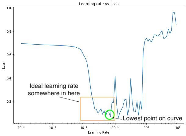
The ideal learning rate at the start of model training is somewhere just before the loss curve bottoms out (a value where the loss is still decreasing).

In [ ]:

# Example of other typical learning rate values
10**0, 10**-1, 10**-2, 10**-3, 1e-4

# Example of other typical learning rate values 10**0, 10**-1, 10**-2, 10**-3, 1e-4

Out[ ]:

(1, 0.1, 0.01, 0.001, 0.0001)

Now we've estimated the ideal learning rate (we'll use 0.02) for our model, let's refit it.

In [ ]:

# Set the random seed
tf.random.set_seed(42)

# Create the model
model_10 = tf.keras.Sequential([
  tf.keras.layers.Dense(4, activation="relu"),
  tf.keras.layers.Dense(4, activation="relu"),
  tf.keras.layers.Dense(1, activation="sigmoid")
])

# Compile the model with the ideal learning rate
model_10.compile(loss="binary_crossentropy",
                optimizer=tf.keras.optimizers.Adam(lr=0.02), # to adjust the learning rate, you need to use tf.keras.optimizers.Adam (not "adam")
                metrics=["accuracy"])

# Fit the model for 20 epochs (5 less than before)
history = model_10.fit(X_train, y_train, epochs=20)

# Set the random seed tf.random.set_seed(42) # Create the model model_10 = tf.keras.Sequential([ tf.keras.layers.Dense(4, activation="relu"), tf.keras.layers.Dense(4, activation="relu"), tf.keras.layers.Dense(1, activation="sigmoid") ]) # Compile the model with the ideal learning rate model_10.compile(loss="binary_crossentropy", optimizer=tf.keras.optimizers.Adam(lr=0.02), # to adjust the learning rate, you need to use tf.keras.optimizers.Adam (not "adam") metrics=["accuracy"]) # Fit the model for 20 epochs (5 less than before) history = model_10.fit(X_train, y_train, epochs=20)

/usr/local/lib/python3.7/dist-packages/keras/optimizer_v2/adam.py:105: UserWarning: The `lr` argument is deprecated, use `learning_rate` instead.
  super(Adam, self).__init__(name, **kwargs)

Epoch 1/20
25/25 [==============================] - 0s 1ms/step - loss: 0.6837 - accuracy: 0.5600
Epoch 2/20
25/25 [==============================] - 0s 1ms/step - loss: 0.6744 - accuracy: 0.5750
Epoch 3/20
25/25 [==============================] - 0s 1ms/step - loss: 0.6626 - accuracy: 0.5875
Epoch 4/20
25/25 [==============================] - 0s 1ms/step - loss: 0.6332 - accuracy: 0.6388
Epoch 5/20
25/25 [==============================] - 0s 2ms/step - loss: 0.5830 - accuracy: 0.7563
Epoch 6/20
25/25 [==============================] - 0s 2ms/step - loss: 0.4907 - accuracy: 0.8313
Epoch 7/20
25/25 [==============================] - 0s 2ms/step - loss: 0.4251 - accuracy: 0.8450
Epoch 8/20
25/25 [==============================] - 0s 2ms/step - loss: 0.3596 - accuracy: 0.8875
Epoch 9/20
25/25 [==============================] - 0s 2ms/step - loss: 0.3152 - accuracy: 0.9100
Epoch 10/20
25/25 [==============================] - 0s 2ms/step - loss: 0.2512 - accuracy: 0.9500
Epoch 11/20
25/25 [==============================] - 0s 2ms/step - loss: 0.2152 - accuracy: 0.9500
Epoch 12/20
25/25 [==============================] - 0s 1ms/step - loss: 0.1721 - accuracy: 0.9750
Epoch 13/20
25/25 [==============================] - 0s 1ms/step - loss: 0.1443 - accuracy: 0.9837
Epoch 14/20
25/25 [==============================] - 0s 2ms/step - loss: 0.1232 - accuracy: 0.9862
Epoch 15/20
25/25 [==============================] - 0s 1ms/step - loss: 0.1085 - accuracy: 0.9850
Epoch 16/20
25/25 [==============================] - 0s 2ms/step - loss: 0.0940 - accuracy: 0.9937
Epoch 17/20
25/25 [==============================] - 0s 2ms/step - loss: 0.0827 - accuracy: 0.9962
Epoch 18/20
25/25 [==============================] - 0s 1ms/step - loss: 0.0798 - accuracy: 0.9937
Epoch 19/20
25/25 [==============================] - 0s 2ms/step - loss: 0.0845 - accuracy: 0.9875
Epoch 20/20
25/25 [==============================] - 0s 2ms/step - loss: 0.0790 - accuracy: 0.9887

Nice! With a little higher learning rate (0.02 instead of 0.01) we reach a higher accuracy than model_8 in less epochs (20 instead of 25).

🛠 Practice: Now you've seen an example of what can happen when you change the learning rate, try changing the learning rate value in the TensorFlow Playground and see what happens. What happens if you increase it? What happens if you decrease it?

In [ ]:

# Evaluate model on the test dataset
model_10.evaluate(X_test, y_test)

# Evaluate model on the test dataset model_10.evaluate(X_test, y_test)

7/7 [==============================] - 0s 3ms/step - loss: 0.0574 - accuracy: 0.9900

Out[ ]:

[0.05740184709429741, 0.9900000095367432]

Let's see how the predictions look.

In [ ]:

# Plot the decision boundaries for the training and test sets
plt.figure(figsize=(12, 6))
plt.subplot(1, 2, 1)
plt.title("Train")
plot_decision_boundary(model_10, X=X_train, y=y_train)
plt.subplot(1, 2, 2)
plt.title("Test")
plot_decision_boundary(model_10, X=X_test, y=y_test)
plt.show()

# Plot the decision boundaries for the training and test sets plt.figure(figsize=(12, 6)) plt.subplot(1, 2, 1) plt.title("Train") plot_decision_boundary(model_10, X=X_train, y=y_train) plt.subplot(1, 2, 2) plt.title("Test") plot_decision_boundary(model_10, X=X_test, y=y_test) plt.show()

doing binary classifcation...
doing binary classifcation...

And as we can see, almost perfect again.

These are the kind of experiments you'll be running often when building your own models.

Start with default settings and see how they perform on your data.

And if they don't perform as well as you'd like, improve them.

Let's look at a few more ways to evaluate our classification models.

More classification evaluation methods¶

Alongside the visualizations we've been making, there are a number of different evaluation metrics we can use to evaluate our classification models.

Metric name/Evaluation method	Defintion	Code
Accuracy	Out of 100 predictions, how many does your model get correct? E.g. 95% accuracy means it gets 95/100 predictions correct.	sklearn.metrics.accuracy_score() or tf.keras.metrics.Accuracy()
Precision	Proportion of true positives over total number of samples. Higher precision leads to less false positives (model predicts 1 when it should've been 0).	sklearn.metrics.precision_score() or tf.keras.metrics.Precision()
Recall	Proportion of true positives over total number of true positives and false negatives (model predicts 0 when it should've been 1). Higher recall leads to less false negatives.	sklearn.metrics.recall_score() or tf.keras.metrics.Recall()
F1-score	Combines precision and recall into one metric. 1 is best, 0 is worst.	sklearn.metrics.f1_score()
Confusion matrix	Compares the predicted values with the true values in a tabular way, if 100% correct, all values in the matrix will be top left to bottom right (diagnol line).	Custom function or sklearn.metrics.plot_confusion_matrix()
Classification report	Collection of some of the main classification metrics such as precision, recall and f1-score.	sklearn.metrics.classification_report()

🔑 Note: Every classification problem will require different kinds of evaluation methods. But you should be familiar with at least the ones above.

Let's start with accuracy.

Because we passed ["accuracy"] to the metrics parameter when we compiled our model, calling evaluate() on it will return the loss as well as accuracy.

In [ ]:

# Check the accuracy of our model
loss, accuracy = model_10.evaluate(X_test, y_test)
print(f"Model loss on test set: {loss}")
print(f"Model accuracy on test set: {(accuracy*100):.2f}%")

# Check the accuracy of our model loss, accuracy = model_10.evaluate(X_test, y_test) print(f"Model loss on test set: {loss}") print(f"Model accuracy on test set: {(accuracy*100):.2f}%")

7/7 [==============================] - 0s 2ms/step - loss: 0.0574 - accuracy: 0.9900
Model loss on test set: 0.05740184709429741
Model accuracy on test set: 99.00%

How about a confusion matrix?

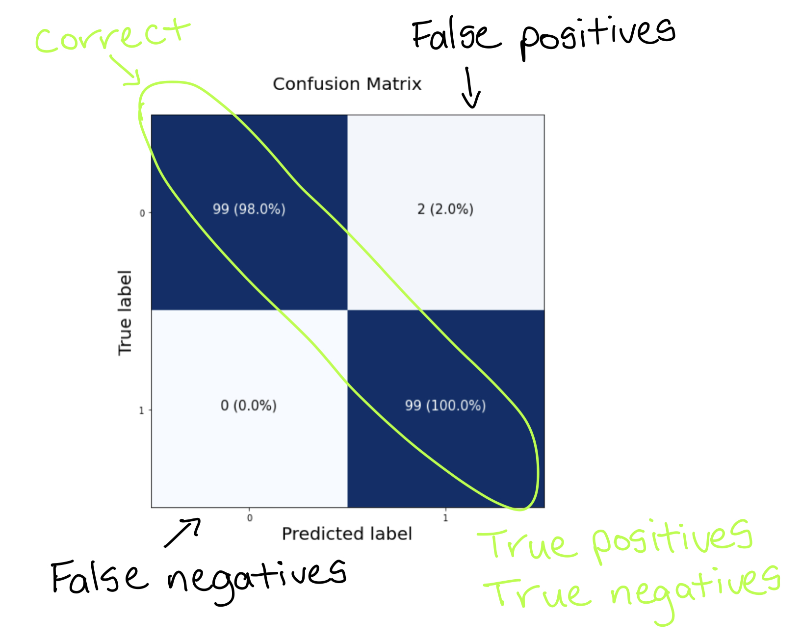Anatomy of a confusion matrix (what we're going to be creating). Correct predictions appear down the diagonal (from top left to bottom right).

We can make a confusion matrix using Scikit-Learn's confusion_matrix method.

In [ ]:

y_test, y_preds

y_test, y_preds

Out[ ]:

(array([1, 1, 1, 1, 0, 0, 1, 0, 1, 0, 1, 0, 1, 1, 1, 1, 1, 1, 0, 1, 0, 1,
        1, 1, 0, 1, 1, 0, 0, 1, 0, 1, 1, 0, 0, 1, 1, 1, 1, 1, 1, 1, 1, 0,
        1, 1, 1, 0, 1, 0, 0, 1, 1, 0, 0, 0, 1, 0, 0, 1, 0, 0, 0, 1, 0, 1,
        0, 0, 0, 0, 1, 0, 1, 1, 1, 1, 0, 1, 0, 0, 0, 0, 0, 0, 1, 0, 1, 0,
        1, 0, 1, 1, 1, 0, 1, 0, 1, 0, 0, 1, 1, 1, 0, 0, 0, 1, 1, 0, 1, 0,
        1, 1, 0, 1, 0, 0, 1, 1, 1, 0, 0, 0, 1, 1, 0, 0, 0, 0, 0, 1, 1, 0,
        1, 0, 0, 0, 1, 0, 0, 0, 1, 1, 1, 1, 0, 1, 1, 1, 0, 1, 1, 1, 1, 0,
        1, 1, 0, 1, 1, 0, 0, 1, 1, 1, 0, 0, 0, 0, 0, 0, 1, 0, 0, 1, 0, 0,
        0, 1, 0, 1, 0, 1, 1, 0, 0, 0, 0, 0, 0, 0, 0, 1, 0, 1, 0, 0, 0, 1,
        0, 0]), array([[9.85265374e-01],
        [9.99237895e-01],
        [9.90323484e-01],
        [9.97069418e-01],
        [3.96229774e-01],
        [1.81269348e-02],
        [9.68290687e-01],
        [1.97467208e-02],
        [9.99671698e-01],
        [5.64604998e-04],
        [9.72873628e-01],
        [2.71522194e-01],
        [9.92272019e-01],
        [9.27265525e-01],
        [9.98101592e-01],
        [9.91818786e-01],
        [9.91739690e-01],
        [9.33626771e-01],
        [4.25938964e-02],
        [9.91493583e-01],
        [1.49991810e-02],
        [9.32794929e-01],
        [9.92896199e-01],
        [9.73198414e-01],
        [4.26525003e-05],
        [9.21439886e-01],
        [9.65749145e-01],
        [2.41607308e-01],
        [1.93991065e-02],
        [9.98130977e-01],
        [1.44242942e-02],
        [9.44148898e-01],
        [9.86896753e-01],
        [1.23808295e-01],
        [2.88016796e-02],
        [9.63382125e-01],
        [9.98146296e-01],
        [9.63414907e-01],
        [9.95050430e-01],
        [9.88492191e-01],
        [9.97049570e-01],
        [9.32708561e-01],
        [9.76667762e-01],
        [9.27743316e-03],
        [9.99066114e-01],
        [9.61072683e-01],
        [9.96635497e-01],
        [1.02143586e-02],
        [9.99359012e-01],
        [3.07261944e-04],
        [3.47039104e-03],
        [9.74120140e-01],
        [9.88394320e-01],
        [8.70075226e-02],
        [1.88689619e-01],
        [9.95191658e-05],
        [9.94503379e-01],
        [4.52136993e-02],
        [2.88990140e-03],
        [9.80903387e-01],
        [8.84046257e-02],
        [7.83565342e-02],
        [5.05689085e-02],
        [9.01162982e-01],
        [2.15362608e-02],
        [9.57937360e-01],
        [6.47488236e-03],
        [7.94454634e-01],
        [8.27848911e-04],
        [1.45462291e-05],
        [9.99163151e-01],
        [1.42278224e-01],
        [9.99482691e-01],
        [9.90508735e-01],
        [9.40230489e-01],
        [9.99421000e-01],
        [4.85877827e-05],
        [9.86135900e-01],
        [2.30431557e-04],
        [1.96249783e-02],
        [2.43693590e-04],
        [3.13844979e-02],
        [2.12577492e-01],
        [1.25015974e-02],
        [5.30756712e-01],
        [4.01511848e-01],
        [9.93256390e-01],
        [1.04149578e-04],
        [9.70202327e-01],
        [5.06452918e-02],
        [9.89271104e-01],
        [9.92339969e-01],
        [9.91254508e-01],
        [5.80731928e-02],
        [9.89033222e-01],
        [1.37410462e-02],
        [9.70293164e-01],
        [1.32769346e-04],
        [1.20589313e-04],
        [9.99783158e-01],
        [9.50982332e-01],
        [9.96350527e-01],
        [8.47944617e-03],
        [6.44198060e-03],
        [1.72309041e-01],
        [9.94098186e-01],
        [9.87757802e-01],
        [4.52793539e-02],
        [9.56778765e-01],
        [1.86411762e-05],
        [9.32023406e-01],
        [9.30726588e-01],
        [5.22510409e-02],
        [9.71138835e-01],
        [2.53470451e-01],
        [2.03959346e-02],
        [9.92558002e-01],
        [9.99580801e-01],
        [9.90525961e-01],
        [1.57394409e-02],
        [3.70688438e-02],
        [6.21199608e-04],
        [9.94643629e-01],
        [9.86936092e-01],
        [2.76437879e-01],
        [2.27220462e-05],
        [6.01140857e-01],
        [1.80983245e-02],
        [4.11799252e-02],
        [9.53140974e-01],
        [9.99358475e-01],
        [3.99774313e-02],
        [9.63670015e-01],
        [5.21329045e-03],
        [1.08969212e-03],
        [2.55343318e-03],
        [9.76243734e-01],
        [5.58070540e-02],
        [1.35067016e-01],
        [6.68315887e-02],
        [9.90237832e-01],
        [9.99417663e-01],
        [9.99269247e-01],
        [9.96144176e-01],
        [1.04406476e-03],
        [9.99343693e-01],
        [9.80513215e-01],
        [9.94254410e-01],
        [9.35024023e-03],
        [9.87102628e-01],
        [9.96918499e-01],
        [9.79749501e-01],
        [9.76329684e-01],
        [9.37545598e-02],
        [9.94555116e-01],
        [9.92427588e-01],
        [1.55746937e-04],
        [9.90727663e-01],
        [9.99703765e-01],
        [7.88568796e-05],
        [1.40845776e-04],
        [9.51246142e-01],
        [9.90273774e-01],
        [9.57789421e-01],
        [1.02409124e-02],
        [1.01274252e-02],
        [2.31212378e-03],
        [3.76697535e-05],
        [3.19328904e-03],
        [1.05946034e-01],
        [9.97693896e-01],
        [1.47536993e-02],
        [5.76236546e-02],
        [9.53175306e-01],
        [4.92044091e-02],
        [1.95735693e-03],
        [2.82667577e-02],
        [9.37708437e-01],
        [1.47617161e-02],
        [9.56363916e-01],
        [1.53975427e-01],
        [9.32425737e-01],
        [9.97206509e-01],
        [6.57788813e-02],
        [1.02413058e-01],
        [6.29435778e-02],
        [1.48057938e-04],
        [2.68450379e-03],
        [1.55602127e-01],
        [1.97130442e-02],
        [4.01784748e-01],
        [9.29691315e-01],
        [5.48276305e-03],
        [9.95398879e-01],
        [1.24812126e-04],
        [8.78109932e-02],
        [1.31530464e-02],
        [9.96485710e-01],
        [6.41274452e-03],
        [3.42636704e-02]], dtype=float32))

In [ ]:

# Create a confusion matrix
from sklearn.metrics import confusion_matrix

# Make predictions
y_preds = model_10.predict(X_test)

# Create confusion matrix
confusion_matrix(y_test, y_preds)

# Create a confusion matrix from sklearn.metrics import confusion_matrix # Make predictions y_preds = model_10.predict(X_test) # Create confusion matrix confusion_matrix(y_test, y_preds)

---------------------------------------------------------------------------
ValueError                                Traceback (most recent call last)
<ipython-input-62-f9843efd97f5> in <module>()
      6 
      7 # Create confusion matrix
----> 8 confusion_matrix(y_test, y_preds)

/usr/local/lib/python3.7/dist-packages/sklearn/metrics/_classification.py in confusion_matrix(y_true, y_pred, labels, sample_weight, normalize)
    305     (0, 2, 1, 1)
    306     """
--> 307     y_type, y_true, y_pred = _check_targets(y_true, y_pred)
    308     if y_type not in ("binary", "multiclass"):
    309         raise ValueError("%s is not supported" % y_type)

/usr/local/lib/python3.7/dist-packages/sklearn/metrics/_classification.py in _check_targets(y_true, y_pred)
     93         raise ValueError(
     94             "Classification metrics can't handle a mix of {0} and {1} targets".format(
---> 95                 type_true, type_pred
     96             )
     97         )

ValueError: Classification metrics can't handle a mix of binary and continuous targets

Ahh, it seems our predictions aren't in the format they need to be.

Let's check them out.

In [ ]:

# View the first 10 predictions
y_preds[:10]

# View the first 10 predictions y_preds[:10]

Out[ ]:

array([[9.8526537e-01],
       [9.9923790e-01],
       [9.9032348e-01],
       [9.9706942e-01],
       [3.9622977e-01],
       [1.8126935e-02],
       [9.6829069e-01],
       [1.9746721e-02],
       [9.9967170e-01],
       [5.6460500e-04]], dtype=float32)

What about our test labels?

In [ ]:

# View the first 10 test labels
y_test[:10]

# View the first 10 test labels y_test[:10]

Out[ ]:

array([1, 1, 1, 1, 0, 0, 1, 0, 1, 0])

It looks like we need to get our predictions into the binary format (0 or 1).

But you might be wondering, what format are they currently in?

In their current format (9.8526537e-01), they're in a form called prediction probabilities.

You'll see this often with the outputs of neural networks. Often they won't be exact values but more a probability of how likely they are to be one value or another.

So one of the steps you'll often see after making predicitons with a neural network is converting the prediction probabilities into labels.

In our case, since our ground truth labels (y_test) are binary (0 or 1), we can convert the prediction probabilities using to their binary form using tf.round().

In [ ]:

# Convert prediction probabilities to binary format and view the first 10
tf.round(y_preds)[:10]

# Convert prediction probabilities to binary format and view the first 10 tf.round(y_preds)[:10]

Out[ ]:

<tf.Tensor: shape=(10, 1), dtype=float32, numpy=
array([[1.],
       [1.],
       [1.],
       [1.],
       [0.],
       [0.],
       [1.],
       [0.],
       [1.],
       [0.]], dtype=float32)>

Wonderful! Now we can use the confusion_matrix function.

In [ ]:

# Create a confusion matrix
confusion_matrix(y_test, tf.round(y_preds))

# Create a confusion matrix confusion_matrix(y_test, tf.round(y_preds))

Out[ ]:

array([[99,  2],
       [ 0, 99]])

Alright, we can see the highest numbers are down the diagonal (from top left to bottom right) so this a good sign, but the rest of the matrix doesn't really tell us much.

How about we make a function to make our confusion matrix a little more visual?

In [ ]:

# Note: The following confusion matrix code is a remix of Scikit-Learn's 
# plot_confusion_matrix function - https://scikit-learn.org/stable/modules/generated/sklearn.metrics.plot_confusion_matrix.html
# and Made with ML's introductory notebook - https://github.com/GokuMohandas/MadeWithML/blob/main/notebooks/08_Neural_Networks.ipynb 
import itertools

figsize = (10, 10)

# Create the confusion matrix
cm = confusion_matrix(y_test, tf.round(y_preds))
cm_norm = cm.astype("float") / cm.sum(axis=1)[:, np.newaxis] # normalize it
n_classes = cm.shape[0]

# Let's prettify it
fig, ax = plt.subplots(figsize=figsize)
# Create a matrix plot
cax = ax.matshow(cm, cmap=plt.cm.Blues) # https://matplotlib.org/3.2.0/api/_as_gen/matplotlib.axes.Axes.matshow.html
fig.colorbar(cax)

# Create classes
classes = False

if classes:
  labels = classes
else:
  labels = np.arange(cm.shape[0])

# Label the axes
ax.set(title="Confusion Matrix",
       xlabel="Predicted label",
       ylabel="True label",
       xticks=np.arange(n_classes),
       yticks=np.arange(n_classes),
       xticklabels=labels,
       yticklabels=labels)

# Set x-axis labels to bottom
ax.xaxis.set_label_position("bottom")
ax.xaxis.tick_bottom()

# Adjust label size
ax.xaxis.label.set_size(20)
ax.yaxis.label.set_size(20)
ax.title.set_size(20)

# Set threshold for different colors
threshold = (cm.max() + cm.min()) / 2.

# Plot the text on each cell
for i, j in itertools.product(range(cm.shape[0]), range(cm.shape[1])):
  plt.text(j, i, f"{cm[i, j]} ({cm_norm[i, j]*100:.1f}%)",
           horizontalalignment="center",
           color="white" if cm[i, j] > threshold else "black",
           size=15)

# Note: The following confusion matrix code is a remix of Scikit-Learn's # plot_confusion_matrix function - https://scikit-learn.org/stable/modules/generated/sklearn.metrics.plot_confusion_matrix.html # and Made with ML's introductory notebook - https://github.com/GokuMohandas/MadeWithML/blob/main/notebooks/08_Neural_Networks.ipynb import itertools figsize = (10, 10) # Create the confusion matrix cm = confusion_matrix(y_test, tf.round(y_preds)) cm_norm = cm.astype("float") / cm.sum(axis=1)[:, np.newaxis] # normalize it n_classes = cm.shape[0] # Let's prettify it fig, ax = plt.subplots(figsize=figsize) # Create a matrix plot cax = ax.matshow(cm, cmap=plt.cm.Blues) # https://matplotlib.org/3.2.0/api/_as_gen/matplotlib.axes.Axes.matshow.html fig.colorbar(cax) # Create classes classes = False if classes: labels = classes else: labels = np.arange(cm.shape[0]) # Label the axes ax.set(title="Confusion Matrix", xlabel="Predicted label", ylabel="True label", xticks=np.arange(n_classes), yticks=np.arange(n_classes), xticklabels=labels, yticklabels=labels) # Set x-axis labels to bottom ax.xaxis.set_label_position("bottom") ax.xaxis.tick_bottom() # Adjust label size ax.xaxis.label.set_size(20) ax.yaxis.label.set_size(20) ax.title.set_size(20) # Set threshold for different colors threshold = (cm.max() + cm.min()) / 2. # Plot the text on each cell for i, j in itertools.product(range(cm.shape[0]), range(cm.shape[1])): plt.text(j, i, f"{cm[i, j]} ({cm_norm[i, j]*100:.1f}%)", horizontalalignment="center", color="white" if cm[i, j] > threshold else "black", size=15)

That looks much better. It seems our model has made almost perfect predictions on the test set except for two false positives (top right corner).

In [ ]:

# What does itertools.product do? Combines two things into each combination
import itertools
for i, j in itertools.product(range(cm.shape[0]), range(cm.shape[1])):
  print(i, j)

# What does itertools.product do? Combines two things into each combination import itertools for i, j in itertools.product(range(cm.shape[0]), range(cm.shape[1])): print(i, j)

0 0
0 1
1 0
1 1

Working with a larger example (multiclass classification)¶

We've seen a binary classification example (predicting if a data point is part of a red circle or blue circle) but what if you had multiple different classes of things?

For example, say you were a fashion company and you wanted to build a neural network to predict whether a piece of clothing was a shoe, a shirt or a jacket (3 different options).

When you have more than two classes as an option, this is known as multiclass classification.

The good news is, the things we've learned so far (with a few tweaks) can be applied to multiclass classification problems as well.

Let's see it in action.

To start, we'll need some data. The good thing for us is TensorFlow has a multiclass classication dataset known as Fashion MNIST built-in. Meaning we can get started straight away.

We can import it using the tf.keras.datasets module.

📖 Resource: The following multiclass classification problem has been adapted from the TensorFlow classification guide. A good exercise would be to once you've gone through the following example, replicate the TensorFlow guide.

In [ ]:

import tensorflow as tf
from tensorflow.keras.datasets import fashion_mnist

# The data has already been sorted into training and test sets for us
(train_data, train_labels), (test_data, test_labels) = fashion_mnist.load_data()

import tensorflow as tf from tensorflow.keras.datasets import fashion_mnist # The data has already been sorted into training and test sets for us (train_data, train_labels), (test_data, test_labels) = fashion_mnist.load_data()

Downloading data from https://storage.googleapis.com/tensorflow/tf-keras-datasets/train-labels-idx1-ubyte.gz
32768/29515 [=================================] - 0s 0us/step
40960/29515 [=========================================] - 0s 0us/step
Downloading data from https://storage.googleapis.com/tensorflow/tf-keras-datasets/train-images-idx3-ubyte.gz
26427392/26421880 [==============================] - 0s 0us/step
26435584/26421880 [==============================] - 0s 0us/step
Downloading data from https://storage.googleapis.com/tensorflow/tf-keras-datasets/t10k-labels-idx1-ubyte.gz
16384/5148 [===============================================================================================] - 0s 0us/step
Downloading data from https://storage.googleapis.com/tensorflow/tf-keras-datasets/t10k-images-idx3-ubyte.gz
4423680/4422102 [==============================] - 0s 0us/step
4431872/4422102 [==============================] - 0s 0us/step

Now let's check out an example.

In [ ]:

# Show the first training example
print(f"Training sample:\n{train_data[0]}\n") 
print(f"Training label: {train_labels[0]}")

# Show the first training example print(f"Training sample:\n{train_data[0]}\n") print(f"Training label: {train_labels[0]}")

Training sample:
[[  0   0   0   0   0   0   0   0   0   0   0   0   0   0   0   0   0   0
    0   0   0   0   0   0   0   0   0   0]
 [  0   0   0   0   0   0   0   0   0   0   0   0   0   0   0   0   0   0
    0   0   0   0   0   0   0   0   0   0]
 [  0   0   0   0   0   0   0   0   0   0   0   0   0   0   0   0   0   0
    0   0   0   0   0   0   0   0   0   0]
 [  0   0   0   0   0   0   0   0   0   0   0   0   1   0   0  13  73   0
    0   1   4   0   0   0   0   1   1   0]
 [  0   0   0   0   0   0   0   0   0   0   0   0   3   0  36 136 127  62
   54   0   0   0   1   3   4   0   0   3]
 [  0   0   0   0   0   0   0   0   0   0   0   0   6   0 102 204 176 134
  144 123  23   0   0   0   0  12  10   0]
 [  0   0   0   0   0   0   0   0   0   0   0   0   0   0 155 236 207 178
  107 156 161 109  64  23  77 130  72  15]
 [  0   0   0   0   0   0   0   0   0   0   0   1   0  69 207 223 218 216
  216 163 127 121 122 146 141  88 172  66]
 [  0   0   0   0   0   0   0   0   0   1   1   1   0 200 232 232 233 229
  223 223 215 213 164 127 123 196 229   0]
 [  0   0   0   0   0   0   0   0   0   0   0   0   0 183 225 216 223 228
  235 227 224 222 224 221 223 245 173   0]
 [  0   0   0   0   0   0   0   0   0   0   0   0   0 193 228 218 213 198
  180 212 210 211 213 223 220 243 202   0]
 [  0   0   0   0   0   0   0   0   0   1   3   0  12 219 220 212 218 192
  169 227 208 218 224 212 226 197 209  52]
 [  0   0   0   0   0   0   0   0   0   0   6   0  99 244 222 220 218 203
  198 221 215 213 222 220 245 119 167  56]
 [  0   0   0   0   0   0   0   0   0   4   0   0  55 236 228 230 228 240
  232 213 218 223 234 217 217 209  92   0]
 [  0   0   1   4   6   7   2   0   0   0   0   0 237 226 217 223 222 219
  222 221 216 223 229 215 218 255  77   0]
 [  0   3   0   0   0   0   0   0   0  62 145 204 228 207 213 221 218 208
  211 218 224 223 219 215 224 244 159   0]
 [  0   0   0   0  18  44  82 107 189 228 220 222 217 226 200 205 211 230
  224 234 176 188 250 248 233 238 215   0]
 [  0  57 187 208 224 221 224 208 204 214 208 209 200 159 245 193 206 223
  255 255 221 234 221 211 220 232 246   0]
 [  3 202 228 224 221 211 211 214 205 205 205 220 240  80 150 255 229 221
  188 154 191 210 204 209 222 228 225   0]
 [ 98 233 198 210 222 229 229 234 249 220 194 215 217 241  65  73 106 117
  168 219 221 215 217 223 223 224 229  29]
 [ 75 204 212 204 193 205 211 225 216 185 197 206 198 213 240 195 227 245
  239 223 218 212 209 222 220 221 230  67]
 [ 48 203 183 194 213 197 185 190 194 192 202 214 219 221 220 236 225 216
  199 206 186 181 177 172 181 205 206 115]
 [  0 122 219 193 179 171 183 196 204 210 213 207 211 210 200 196 194 191
  195 191 198 192 176 156 167 177 210  92]
 [  0   0  74 189 212 191 175 172 175 181 185 188 189 188 193 198 204 209
  210 210 211 188 188 194 192 216 170   0]
 [  2   0   0   0  66 200 222 237 239 242 246 243 244 221 220 193 191 179
  182 182 181 176 166 168  99  58   0   0]
 [  0   0   0   0   0   0   0  40  61  44  72  41  35   0   0   0   0   0
    0   0   0   0   0   0   0   0   0   0]
 [  0   0   0   0   0   0   0   0   0   0   0   0   0   0   0   0   0   0
    0   0   0   0   0   0   0   0   0   0]
 [  0   0   0   0   0   0   0   0   0   0   0   0   0   0   0   0   0   0
    0   0   0   0   0   0   0   0   0   0]]

Training label: 9

Woah, we get a large list of numbers, followed (the data) by a single number (the class label).

What about the shapes?

In [ ]:

# Check the shape of our data
train_data.shape, train_labels.shape, test_data.shape, test_labels.shape

# Check the shape of our data train_data.shape, train_labels.shape, test_data.shape, test_labels.shape

Out[ ]:

((60000, 28, 28), (60000,), (10000, 28, 28), (10000,))

In [ ]:

# Check shape of a single example
train_data[0].shape, train_labels[0].shape

# Check shape of a single example train_data[0].shape, train_labels[0].shape

Out[ ]:

((28, 28), ())

Okay, 60,000 training examples each with shape (28, 28) and a label each as well as 10,000 test examples of shape (28, 28).

But these are just numbers, let's visualize.

In [ ]:

# Plot a single example
import matplotlib.pyplot as plt
plt.imshow(train_data[7]);

# Plot a single example import matplotlib.pyplot as plt plt.imshow(train_data[7]);

Hmm, but what about its label?

In [ ]:

# Check our samples label
train_labels[7]

# Check our samples label train_labels[7]

Out[ ]:

2

It looks like our labels are in numerical form. And while this is fine for a neural network, you might want to have them in human readable form.

Let's create a small list of the class names (we can find them on the dataset's GitHub page).

🔑 Note: Whilst this dataset has been prepared for us and ready to go, it's important to remember many datasets won't be ready to go like this one. Often you'll have to do a few preprocessing steps to have it ready to use with a neural network (we'll see more of this when we work with our own data later).

In [ ]:

class_names = ['T-shirt/top', 'Trouser', 'Pullover', 'Dress', 'Coat', 
               'Sandal', 'Shirt', 'Sneaker', 'Bag', 'Ankle boot']

# How many classes are there (this'll be our output shape)?
len(class_names)

class_names = ['T-shirt/top', 'Trouser', 'Pullover', 'Dress', 'Coat', 'Sandal', 'Shirt', 'Sneaker', 'Bag', 'Ankle boot'] # How many classes are there (this'll be our output shape)? len(class_names)

Out[ ]:

10

Now we have these, let's plot another example.

🤔 Question: Pay particular attention to what the data we're working with looks like. Is it only straight lines? Or does it have non-straight lines as well? Do you think if we wanted to find patterns in the photos of clothes (which are actually collections of pixels), will our model need non-linearities (non-straight lines) or not?

In [ ]:

# Plot an example image and its label
plt.imshow(train_data[17], cmap=plt.cm.binary) # change the colours to black & white
plt.title(class_names[train_labels[17]]);

# Plot an example image and its label plt.imshow(train_data[17], cmap=plt.cm.binary) # change the colours to black & white plt.title(class_names[train_labels[17]]);

In [ ]:

# Plot multiple random images of fashion MNIST
import random
plt.figure(figsize=(7, 7))
for i in range(4):
  ax = plt.subplot(2, 2, i + 1)
  rand_index = random.choice(range(len(train_data)))
  plt.imshow(train_data[rand_index], cmap=plt.cm.binary)
  plt.title(class_names[train_labels[rand_index]])
  plt.axis(False)

# Plot multiple random images of fashion MNIST import random plt.figure(figsize=(7, 7)) for i in range(4): ax = plt.subplot(2, 2, i + 1) rand_index = random.choice(range(len(train_data))) plt.imshow(train_data[rand_index], cmap=plt.cm.binary) plt.title(class_names[train_labels[rand_index]]) plt.axis(False)

Alright, let's build a model to figure out the relationship between the pixel values and their labels.

Since this is a multiclass classification problem, we'll need to make a few changes to our architecture (inline with Table 1 above):

• The input shape will have to deal with 28x28 tensors (the height and width of our images).
  • We're actually going to squash the input into a tensor (vector) of shape (784).
• The output shape will have to be 10 because we need our model to predict for 10 different classes.
  • We'll also change the activation parameter of our output layer to be "softmax" instead of 'sigmoid'. As we'll see the "softmax" activation function outputs a series of values between 0 & 1 (the same shape as output shape, which together add up to ~1. The index with the highest value is predicted by the model to be the most likely class.
• We'll need to change our loss function from a binary loss function to a multiclass loss function.
  • More specifically, since our labels are in integer form, we'll use tf.keras.losses.SparseCategoricalCrossentropy(), if our labels were one-hot encoded (e.g. they looked something like [0, 0, 1, 0, 0...]), we'd use tf.keras.losses.CategoricalCrossentropy().
• We'll also use the validation_data parameter when calling the fit() function. This will give us an idea of how the model performs on the test set during training.

You ready? Let's go.

In [ ]:

# Set random seed
tf.random.set_seed(42)

# Create the model
model_11 = tf.keras.Sequential([
  tf.keras.layers.Flatten(input_shape=(28, 28)), # input layer (we had to reshape 28x28 to 784, the Flatten layer does this for us)
  tf.keras.layers.Dense(4, activation="relu"),
  tf.keras.layers.Dense(4, activation="relu"),
  tf.keras.layers.Dense(10, activation="softmax") # output shape is 10, activation is softmax
])

# Compile the model
model_11.compile(loss=tf.keras.losses.SparseCategoricalCrossentropy(), # different loss function for multiclass classifcation
                 optimizer=tf.keras.optimizers.Adam(),
                 metrics=["accuracy"])

# Fit the model
non_norm_history = model_11.fit(train_data,
                                train_labels,
                                epochs=10,
                                validation_data=(test_data, test_labels)) # see how the model performs on the test set during training

# Set random seed tf.random.set_seed(42) # Create the model model_11 = tf.keras.Sequential([ tf.keras.layers.Flatten(input_shape=(28, 28)), # input layer (we had to reshape 28x28 to 784, the Flatten layer does this for us) tf.keras.layers.Dense(4, activation="relu"), tf.keras.layers.Dense(4, activation="relu"), tf.keras.layers.Dense(10, activation="softmax") # output shape is 10, activation is softmax ]) # Compile the model model_11.compile(loss=tf.keras.losses.SparseCategoricalCrossentropy(), # different loss function for multiclass classifcation optimizer=tf.keras.optimizers.Adam(), metrics=["accuracy"]) # Fit the model non_norm_history = model_11.fit(train_data, train_labels, epochs=10, validation_data=(test_data, test_labels)) # see how the model performs on the test set during training

Epoch 1/10
1875/1875 [==============================] - 5s 3ms/step - loss: 2.1671 - accuracy: 0.1606 - val_loss: 1.7959 - val_accuracy: 0.2046
Epoch 2/10
1875/1875 [==============================] - 4s 2ms/step - loss: 1.7066 - accuracy: 0.2509 - val_loss: 1.6567 - val_accuracy: 0.2805
Epoch 3/10
1875/1875 [==============================] - 4s 2ms/step - loss: 1.6321 - accuracy: 0.2806 - val_loss: 1.6094 - val_accuracy: 0.2857
Epoch 4/10
1875/1875 [==============================] - 4s 2ms/step - loss: 1.6052 - accuracy: 0.2833 - val_loss: 1.6041 - val_accuracy: 0.2859
Epoch 5/10
1875/1875 [==============================] - 4s 2ms/step - loss: 1.5975 - accuracy: 0.2862 - val_loss: 1.6064 - val_accuracy: 0.2756
Epoch 6/10
1875/1875 [==============================] - 4s 2ms/step - loss: 1.5950 - accuracy: 0.2920 - val_loss: 1.5747 - val_accuracy: 0.2994
Epoch 7/10
1875/1875 [==============================] - 4s 2ms/step - loss: 1.5775 - accuracy: 0.3040 - val_loss: 1.6030 - val_accuracy: 0.3000
Epoch 8/10
1875/1875 [==============================] - 4s 2ms/step - loss: 1.5708 - accuracy: 0.3175 - val_loss: 1.5635 - val_accuracy: 0.3315
Epoch 9/10
1875/1875 [==============================] - 4s 2ms/step - loss: 1.5638 - accuracy: 0.3280 - val_loss: 1.5534 - val_accuracy: 0.3334
Epoch 10/10
1875/1875 [==============================] - 4s 2ms/step - loss: 1.5432 - accuracy: 0.3346 - val_loss: 1.5390 - val_accuracy: 0.3549

In [ ]:

# Check the shapes of our model
# Note: the "None" in (None, 784) is for batch_size, we'll cover this in a later module
model_11.summary()

# Check the shapes of our model # Note: the "None" in (None, 784) is for batch_size, we'll cover this in a later module model_11.summary()

Alright, our model gets to about ~35% accuracy after 10 epochs using a similar style model to what we used on our binary classification problem.

Which is better than guessing (guessing with 10 classes would result in about 10% accuracy) but we can do better.

Do you remember when we talked about neural networks preferring numbers between 0 and 1? (if not, treat this as a reminder)

Well, right now, the data we have isn't between 0 and 1, in other words, it's not normalized (hence why we used the non_norm_history variable when calling fit()). It's pixel values are between 0 and 255.

Let's see.

In [ ]:

# Check the min and max values of the training data
train_data.min(), train_data.max()

# Check the min and max values of the training data train_data.min(), train_data.max()

We can get these values between 0 and 1 by dividing the entire array by the maximum: 255.0 (dividing by a float also converts to a float).

Doing so will result in all of our data being between 0 and 1 (known as scaling or normalization).

In [ ]:

# Divide train and test images by the maximum value (normalize it)
train_data = train_data / 255.0
test_data = test_data / 255.0

# Check the min and max values of the training data
train_data.min(), train_data.max()

# Divide train and test images by the maximum value (normalize it) train_data = train_data / 255.0 test_data = test_data / 255.0 # Check the min and max values of the training data train_data.min(), train_data.max()

Beautiful! Now our data is between 0 and 1. Let's see what happens when we model it.

We'll use the same model as before (model_11) except this time the data will be normalized.

In [ ]:

# Set random seed
tf.random.set_seed(42)

# Create the model
model_12 = tf.keras.Sequential([
  tf.keras.layers.Flatten(input_shape=(28, 28)), # input layer (we had to reshape 28x28 to 784)
  tf.keras.layers.Dense(4, activation="relu"),
  tf.keras.layers.Dense(4, activation="relu"),
  tf.keras.layers.Dense(10, activation="softmax") # output shape is 10, activation is softmax
])

# Compile the model
model_12.compile(loss=tf.keras.losses.SparseCategoricalCrossentropy(),
                 optimizer=tf.keras.optimizers.Adam(),
                 metrics=["accuracy"])

# Fit the model (to the normalized data)
norm_history = model_12.fit(train_data,
                            train_labels,
                            epochs=10,
                            validation_data=(test_data, test_labels))

# Set random seed tf.random.set_seed(42) # Create the model model_12 = tf.keras.Sequential([ tf.keras.layers.Flatten(input_shape=(28, 28)), # input layer (we had to reshape 28x28 to 784) tf.keras.layers.Dense(4, activation="relu"), tf.keras.layers.Dense(4, activation="relu"), tf.keras.layers.Dense(10, activation="softmax") # output shape is 10, activation is softmax ]) # Compile the model model_12.compile(loss=tf.keras.losses.SparseCategoricalCrossentropy(), optimizer=tf.keras.optimizers.Adam(), metrics=["accuracy"]) # Fit the model (to the normalized data) norm_history = model_12.fit(train_data, train_labels, epochs=10, validation_data=(test_data, test_labels))

Woah, we used the exact same model as before but we with normalized data we're now seeing a much higher accuracy value!

Let's plot each model's history (their loss curves).

In [ ]:

import pandas as pd
# Plot non-normalized data loss curves
pd.DataFrame(non_norm_history.history).plot(title="Non-normalized Data")
# Plot normalized data loss curves
pd.DataFrame(norm_history.history).plot(title="Normalized data");

import pandas as pd # Plot non-normalized data loss curves pd.DataFrame(non_norm_history.history).plot(title="Non-normalized Data") # Plot normalized data loss curves pd.DataFrame(norm_history.history).plot(title="Normalized data");

Wow. From these two plots, we can see how much quicker our model with the normalized data (model_12) improved than the model with the non-normalized data (model_11).

🔑 Note: The same model with even slightly different data can produce dramatically different results. So when you're comparing models, it's important to make sure you're comparing them on the same criteria (e.g. same architecture but different data or same data but different architecture).

How about we find the ideal learning rate and see what happens?

We'll use the same architecture we've been using.

In [ ]:

# Set random seed
tf.random.set_seed(42)

# Create the model
model_13 = tf.keras.Sequential([
  tf.keras.layers.Flatten(input_shape=(28, 28)), # input layer (we had to reshape 28x28 to 784)
  tf.keras.layers.Dense(4, activation="relu"),
  tf.keras.layers.Dense(4, activation="relu"),
  tf.keras.layers.Dense(10, activation="softmax") # output shape is 10, activation is softmax
])

# Compile the model
model_13.compile(loss=tf.keras.losses.SparseCategoricalCrossentropy(),
                 optimizer=tf.keras.optimizers.Adam(),
                 metrics=["accuracy"])

# Create the learning rate callback
lr_scheduler = tf.keras.callbacks.LearningRateScheduler(lambda epoch: 1e-3 * 10**(epoch/20))

# Fit the model
find_lr_history = model_13.fit(train_data,
                               train_labels,
                               epochs=40, # model already doing pretty good with current LR, probably don't need 100 epochs
                               validation_data=(test_data, test_labels),
                               callbacks=[lr_scheduler])

# Set random seed tf.random.set_seed(42) # Create the model model_13 = tf.keras.Sequential([ tf.keras.layers.Flatten(input_shape=(28, 28)), # input layer (we had to reshape 28x28 to 784) tf.keras.layers.Dense(4, activation="relu"), tf.keras.layers.Dense(4, activation="relu"), tf.keras.layers.Dense(10, activation="softmax") # output shape is 10, activation is softmax ]) # Compile the model model_13.compile(loss=tf.keras.losses.SparseCategoricalCrossentropy(), optimizer=tf.keras.optimizers.Adam(), metrics=["accuracy"]) # Create the learning rate callback lr_scheduler = tf.keras.callbacks.LearningRateScheduler(lambda epoch: 1e-3 * 10**(epoch/20)) # Fit the model find_lr_history = model_13.fit(train_data, train_labels, epochs=40, # model already doing pretty good with current LR, probably don't need 100 epochs validation_data=(test_data, test_labels), callbacks=[lr_scheduler])

In [ ]:

# Plot the learning rate decay curve
import numpy as np
import matplotlib.pyplot as plt
lrs = 1e-3 * (10**(np.arange(40)/20))
plt.semilogx(lrs, find_lr_history.history["loss"]) # want the x-axis to be log-scale
plt.xlabel("Learning rate")
plt.ylabel("Loss")
plt.title("Finding the ideal learning rate");

# Plot the learning rate decay curve import numpy as np import matplotlib.pyplot as plt lrs = 1e-3 * (10**(np.arange(40)/20)) plt.semilogx(lrs, find_lr_history.history["loss"]) # want the x-axis to be log-scale plt.xlabel("Learning rate") plt.ylabel("Loss") plt.title("Finding the ideal learning rate");

In this case, it looks like somewhere close to the default learning rate of the Adam optimizer (0.001) is the ideal learning rate.

Let's refit a model using the ideal learning rate.

In [ ]:

# Set random seed
tf.random.set_seed(42)

# Create the model
model_14 = tf.keras.Sequential([
  tf.keras.layers.Flatten(input_shape=(28, 28)), # input layer (we had to reshape 28x28 to 784)
  tf.keras.layers.Dense(4, activation="relu"),
  tf.keras.layers.Dense(4, activation="relu"),
  tf.keras.layers.Dense(10, activation="softmax") # output shape is 10, activation is softmax
])

# Compile the model
model_14.compile(loss=tf.keras.losses.SparseCategoricalCrossentropy(),
                 optimizer=tf.keras.optimizers.Adam(lr=0.001), # ideal learning rate (same as default)
                 metrics=["accuracy"])

# Fit the model
history = model_14.fit(train_data,
                       train_labels,
                       epochs=20,
                       validation_data=(test_data, test_labels))

# Set random seed tf.random.set_seed(42) # Create the model model_14 = tf.keras.Sequential([ tf.keras.layers.Flatten(input_shape=(28, 28)), # input layer (we had to reshape 28x28 to 784) tf.keras.layers.Dense(4, activation="relu"), tf.keras.layers.Dense(4, activation="relu"), tf.keras.layers.Dense(10, activation="softmax") # output shape is 10, activation is softmax ]) # Compile the model model_14.compile(loss=tf.keras.losses.SparseCategoricalCrossentropy(), optimizer=tf.keras.optimizers.Adam(lr=0.001), # ideal learning rate (same as default) metrics=["accuracy"]) # Fit the model history = model_14.fit(train_data, train_labels, epochs=20, validation_data=(test_data, test_labels))

Now we've got a model trained with a close-to-ideal learning rate and performing pretty well, we've got a couple of options.

We could:

• Evaluate its performance using other classification metrics (such as a confusion matrix or classification report).
• Assess some of its predictions (through visualizations).
• Improve its accuracy (by training it for longer or changing the architecture).
• Save and export it for use in an application.

Let's go through the first two options.

First we'll create a classification matrix to visualize its predictions across the different classes.

In [ ]:

# Note: The following confusion matrix code is a remix of Scikit-Learn's 
# plot_confusion_matrix function - https://scikit-learn.org/stable/modules/generated/sklearn.metrics.plot_confusion_matrix.html
# and Made with ML's introductory notebook - https://github.com/GokuMohandas/MadeWithML/blob/main/notebooks/08_Neural_Networks.ipynb
import itertools
from sklearn.metrics import confusion_matrix

# Our function needs a different name to sklearn's plot_confusion_matrix
def make_confusion_matrix(y_true, y_pred, classes=None, figsize=(10, 10), text_size=15): 
  """Makes a labelled confusion matrix comparing predictions and ground truth labels.

  If classes is passed, confusion matrix will be labelled, if not, integer class values
  will be used.

  Args:
    y_true: Array of truth labels (must be same shape as y_pred).
    y_pred: Array of predicted labels (must be same shape as y_true).
    classes: Array of class labels (e.g. string form). If `None`, integer labels are used.
    figsize: Size of output figure (default=(10, 10)).
    text_size: Size of output figure text (default=15).
  
  Returns:
    A labelled confusion matrix plot comparing y_true and y_pred.

  Example usage:
    make_confusion_matrix(y_true=test_labels, # ground truth test labels
                          y_pred=y_preds, # predicted labels
                          classes=class_names, # array of class label names
                          figsize=(15, 15),
                          text_size=10)
  """  
  # Create the confustion matrix
  cm = confusion_matrix(y_true, y_pred)
  cm_norm = cm.astype("float") / cm.sum(axis=1)[:, np.newaxis] # normalize it
  n_classes = cm.shape[0] # find the number of classes we're dealing with

  # Plot the figure and make it pretty
  fig, ax = plt.subplots(figsize=figsize)
  cax = ax.matshow(cm, cmap=plt.cm.Blues) # colors will represent how 'correct' a class is, darker == better
  fig.colorbar(cax)

  # Are there a list of classes?
  if classes:
    labels = classes
  else:
    labels = np.arange(cm.shape[0])
  
  # Label the axes
  ax.set(title="Confusion Matrix",
         xlabel="Predicted label",
         ylabel="True label",
         xticks=np.arange(n_classes), # create enough axis slots for each class
         yticks=np.arange(n_classes), 
         xticklabels=labels, # axes will labeled with class names (if they exist) or ints
         yticklabels=labels)
  
  # Make x-axis labels appear on bottom
  ax.xaxis.set_label_position("bottom")
  ax.xaxis.tick_bottom()

  # Set the threshold for different colors
  threshold = (cm.max() + cm.min()) / 2.

  # Plot the text on each cell
  for i, j in itertools.product(range(cm.shape[0]), range(cm.shape[1])):
    plt.text(j, i, f"{cm[i, j]} ({cm_norm[i, j]*100:.1f}%)",
             horizontalalignment="center",
             color="white" if cm[i, j] > threshold else "black",
             size=text_size)

# Note: The following confusion matrix code is a remix of Scikit-Learn's # plot_confusion_matrix function - https://scikit-learn.org/stable/modules/generated/sklearn.metrics.plot_confusion_matrix.html # and Made with ML's introductory notebook - https://github.com/GokuMohandas/MadeWithML/blob/main/notebooks/08_Neural_Networks.ipynb import itertools from sklearn.metrics import confusion_matrix # Our function needs a different name to sklearn's plot_confusion_matrix def make_confusion_matrix(y_true, y_pred, classes=None, figsize=(10, 10), text_size=15): """Makes a labelled confusion matrix comparing predictions and ground truth labels. If classes is passed, confusion matrix will be labelled, if not, integer class values will be used. Args: y_true: Array of truth labels (must be same shape as y_pred). y_pred: Array of predicted labels (must be same shape as y_true). classes: Array of class labels (e.g. string form). If `None`, integer labels are used. figsize: Size of output figure (default=(10, 10)). text_size: Size of output figure text (default=15). Returns: A labelled confusion matrix plot comparing y_true and y_pred. Example usage: make_confusion_matrix(y_true=test_labels, # ground truth test labels y_pred=y_preds, # predicted labels classes=class_names, # array of class label names figsize=(15, 15), text_size=10) """ # Create the confustion matrix cm = confusion_matrix(y_true, y_pred) cm_norm = cm.astype("float") / cm.sum(axis=1)[:, np.newaxis] # normalize it n_classes = cm.shape[0] # find the number of classes we're dealing with # Plot the figure and make it pretty fig, ax = plt.subplots(figsize=figsize) cax = ax.matshow(cm, cmap=plt.cm.Blues) # colors will represent how 'correct' a class is, darker == better fig.colorbar(cax) # Are there a list of classes? if classes: labels = classes else: labels = np.arange(cm.shape[0]) # Label the axes ax.set(title="Confusion Matrix", xlabel="Predicted label", ylabel="True label", xticks=np.arange(n_classes), # create enough axis slots for each class yticks=np.arange(n_classes), xticklabels=labels, # axes will labeled with class names (if they exist) or ints yticklabels=labels) # Make x-axis labels appear on bottom ax.xaxis.set_label_position("bottom") ax.xaxis.tick_bottom() # Set the threshold for different colors threshold = (cm.max() + cm.min()) / 2. # Plot the text on each cell for i, j in itertools.product(range(cm.shape[0]), range(cm.shape[1])): plt.text(j, i, f"{cm[i, j]} ({cm_norm[i, j]*100:.1f}%)", horizontalalignment="center", color="white" if cm[i, j] > threshold else "black", size=text_size)

Since a confusion matrix compares the truth labels (test_labels) to the predicted labels, we have to make some predictions with our model.

In [ ]:

# Make predictions with the most recent model
y_probs = model_14.predict(test_data) # "probs" is short for probabilities

# View the first 5 predictions
y_probs[:5]

# Make predictions with the most recent model y_probs = model_14.predict(test_data) # "probs" is short for probabilities # View the first 5 predictions y_probs[:5]

Our model outputs a list of prediction probabilities, meaning, it outputs a number for how likely it thinks a particular class is to be the label.

The higher the number in the prediction probabilities list, the more likely the model believes that is the right class.

To find the highest value we can use the argmax() method.

In [ ]:

# See the predicted class number and label for the first example
y_probs[0].argmax(), class_names[y_probs[0].argmax()]

# See the predicted class number and label for the first example y_probs[0].argmax(), class_names[y_probs[0].argmax()]

Now let's do the same for all of the predictions.

In [ ]:

# Convert all of the predictions from probabilities to labels
y_preds = y_probs.argmax(axis=1)

# View the first 10 prediction labels
y_preds[:10]

# Convert all of the predictions from probabilities to labels y_preds = y_probs.argmax(axis=1) # View the first 10 prediction labels y_preds[:10]

Wonderful, now we've got our model's predictions in label form, let's create a confusion matrix to view them against the truth labels.

In [ ]:

# Check out the non-prettified confusion matrix
from sklearn.metrics import confusion_matrix
confusion_matrix(y_true=test_labels, 
                 y_pred=y_preds)

# Check out the non-prettified confusion matrix from sklearn.metrics import confusion_matrix confusion_matrix(y_true=test_labels, y_pred=y_preds)

That confusion matrix is hard to comprehend, let's make it prettier using the function we created before.

In [ ]:

# Make a prettier confusion matrix
make_confusion_matrix(y_true=test_labels, 
                      y_pred=y_preds,
                      classes=class_names,
                      figsize=(15, 15),
                      text_size=10)

# Make a prettier confusion matrix make_confusion_matrix(y_true=test_labels, y_pred=y_preds, classes=class_names, figsize=(15, 15), text_size=10)

That looks much better! (one of my favourites sights in the world is a confusion matrix with dark squares down the diagonal)

Except the results aren't as good as they could be...

It looks like our model is getting confused between the Shirt and T-shirt/top classes (e.g. predicting Shirt when it's actually a T-shirt/top).

🤔 Question: Does it make sense that our model is getting confused between the Shirt and T-shirt/top classes? Why do you think this might be? What's one way you could investigate?

We've seen how our models predictions line up to the truth labels using a confusion matrix, but how about we visualize some?

Let's create a function to plot a random image along with its prediction.

🔑 Note: Often when working with images and other forms of visual data, it's a good idea to visualize as much as possible to develop a further understanding of the data and the outputs of your model.

In [ ]:

import random

# Create a function for plotting a random image along with its prediction
def plot_random_image(model, images, true_labels, classes):
  """Picks a random image, plots it and labels it with a predicted and truth label.

  Args:
    model: a trained model (trained on data similar to what's in images).
    images: a set of random images (in tensor form).
    true_labels: array of ground truth labels for images.
    classes: array of class names for images.
  
  Returns:
    A plot of a random image from `images` with a predicted class label from `model`
    as well as the truth class label from `true_labels`.
  """ 
  # Setup random integer
  i = random.randint(0, len(images))
  
  # Create predictions and targets
  target_image = images[i]
  pred_probs = model.predict(target_image.reshape(1, 28, 28)) # have to reshape to get into right size for model
  pred_label = classes[pred_probs.argmax()]
  true_label = classes[true_labels[i]]

  # Plot the target image
  plt.imshow(target_image, cmap=plt.cm.binary)

  # Change the color of the titles depending on if the prediction is right or wrong
  if pred_label == true_label:
    color = "green"
  else:
    color = "red"

  # Add xlabel information (prediction/true label)
  plt.xlabel("Pred: {} {:2.0f}% (True: {})".format(pred_label,
                                                   100*tf.reduce_max(pred_probs),
                                                   true_label),
             color=color) # set the color to green or red

import random # Create a function for plotting a random image along with its prediction def plot_random_image(model, images, true_labels, classes): """Picks a random image, plots it and labels it with a predicted and truth label. Args: model: a trained model (trained on data similar to what's in images). images: a set of random images (in tensor form). true_labels: array of ground truth labels for images. classes: array of class names for images. Returns: A plot of a random image from `images` with a predicted class label from `model` as well as the truth class label from `true_labels`. """ # Setup random integer i = random.randint(0, len(images)) # Create predictions and targets target_image = images[i] pred_probs = model.predict(target_image.reshape(1, 28, 28)) # have to reshape to get into right size for model pred_label = classes[pred_probs.argmax()] true_label = classes[true_labels[i]] # Plot the target image plt.imshow(target_image, cmap=plt.cm.binary) # Change the color of the titles depending on if the prediction is right or wrong if pred_label == true_label: color = "green" else: color = "red" # Add xlabel information (prediction/true label) plt.xlabel("Pred: {} {:2.0f}% (True: {})".format(pred_label, 100*tf.reduce_max(pred_probs), true_label), color=color) # set the color to green or red

In [ ]:

# Check out a random image as well as its prediction
plot_random_image(model=model_14, 
                  images=test_data, 
                  true_labels=test_labels, 
                  classes=class_names)

# Check out a random image as well as its prediction plot_random_image(model=model_14, images=test_data, true_labels=test_labels, classes=class_names)

After running the cell above a few times you'll start to get a visual understanding of the relationship between the model's predictions and the true labels.

Did you figure out which predictions the model gets confused on?

It seems to mix up classes which are similar, for example, Sneaker with Ankle boot.

Looking at the images, you can see how this might be the case.

The overall shape of a Sneaker and an Ankle Boot are similar.

The overall shape might be one of the patterns the model has learned and so therefore when two images have a similar shape, their predictions get mixed up.

What patterns is our model learning?¶

We've been talking a lot about how a neural network finds patterns in numbers, but what exactly do these patterns look like?

Let's crack open one of our models and find out.

First, we'll get a list of layers in our most recent model (model_14) using the layers attribute.

In [ ]:

# Find the layers of our most recent model
model_14.layers

# Find the layers of our most recent model model_14.layers

We can access a target layer using indexing.

In [ ]:

# Extract a particular layer
model_14.layers[1]

# Extract a particular layer model_14.layers[1]

And we can find the patterns learned by a particular layer using the get_weights() method.

The get_weights() method returns the weights (also known as a weights matrix) and biases (also known as a bias vector) of a particular layer.

In [ ]:

# Get the patterns of a layer in our network
weights, biases = model_14.layers[1].get_weights()

# Shape = 1 weight matrix the size of our input data (28x28) per neuron (4)
weights, weights.shape

# Get the patterns of a layer in our network weights, biases = model_14.layers[1].get_weights() # Shape = 1 weight matrix the size of our input data (28x28) per neuron (4) weights, weights.shape

The weights matrix is the same shape as the input data, which in our case is 784 (28x28 pixels). And there's a copy of the weights matrix for each neuron the in the selected layer (our selected layer has 4 neurons).

Each value in the weights matrix corresponds to how a particular value in the input data influences the network's decisions.

These values start out as random numbers (they're set by the kernel_initializer parameter when creating a layer, the default is "glorot_uniform") and are then updated to better representative values of the data (non-random) by the neural network during training.

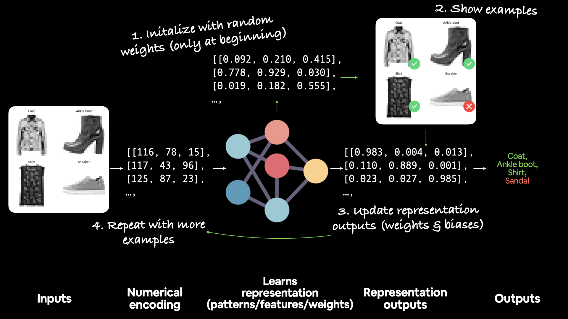Example workflow of how a supervised neural network starts with random weights and updates them to better represent the data by looking at examples of ideal outputs.

Now let's check out the bias vector.

In [ ]:

# Shape = 1 bias per neuron (we use 4 neurons in the first layer)
biases, biases.shape

# Shape = 1 bias per neuron (we use 4 neurons in the first layer) biases, biases.shape

Every neuron has a bias vector. Each of these is paired with a weight matrix.

The bias values get initialized as zeroes by default (using the bias_initializer parameter).

The bias vector dictates how much the patterns within the corresponding weights matrix should influence the next layer.

In [ ]:

# Can now calculate the number of paramters in our model
model_14.summary()

# Can now calculate the number of paramters in our model model_14.summary()

Now we've built a few deep learning models, it's a good time to point out the whole concept of inputs and outputs not only relates to a model as a whole but to every layer within a model.

You might've already guessed this, but starting from the input layer, each subsequent layer's input is the output of the previous layer.

We can see this clearly using the utility plot_model().

In [ ]:

from tensorflow.keras.utils import plot_model

# See the inputs and outputs of each layer
plot_model(model_14, show_shapes=True)

from tensorflow.keras.utils import plot_model # See the inputs and outputs of each layer plot_model(model_14, show_shapes=True)

How a model learns (in brief)¶

Alright, we've trained a bunch of models, but we've never really discussed what's going on under the hood. So how exactly does a model learn?

A model learns by updating and improving its weight matrices and biases values every epoch (in our case, when we call the fit() fucntion).

It does so by comparing the patterns its learned between the data and labels to the actual labels.

If the current patterns (weight matrices and bias values) don't result in a desirable decrease in the loss function (higher loss means worse predictions), the optimizer tries to steer the model to update its patterns in the right way (using the real labels as a reference).

This process of using the real labels as a reference to improve the model's predictions is called backpropagation.

In other words, data and labels pass through a model (forward pass) and it attempts to learn the relationship between the data and labels.

And if this learned relationship isn't close to the actual relationship or it could be improved, the model does so by going back through itself (backward pass) and tweaking its weights matrices and bias values to better represent the data.

If all of this sounds confusing (and it's fine if it does, the above is a very succinct description), check out the resources in the extra-curriculum section for more.

Exercises 🛠¶

1. Play with neural networks in the TensorFlow Playground for 10-minutes. Especially try different values of the learning, what happens when you decrease it? What happens when you increase it?
2. Replicate the model pictured in the TensorFlow Playground diagram below using TensorFlow code. Compile it using the Adam optimizer, binary crossentropy loss and accuracy metric. Once it's compiled check a summary of the model. 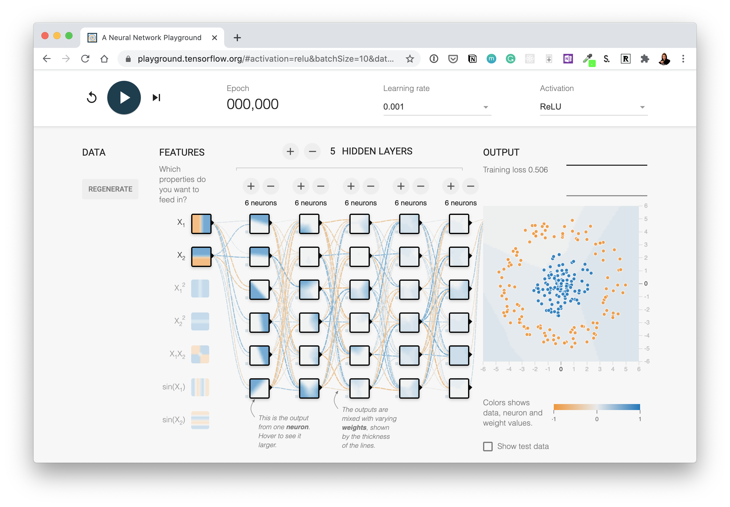Try this network out for yourself on the TensorFlow Playground website. Hint: there are 5 hidden layers but the output layer isn't pictured, you'll have to decide what the output layer should be based on the input data.
3. Create a classification dataset using Scikit-Learn's make_moons() function, visualize it and then build a model to fit it at over 85% accuracy.
4. Create a function (or write code) to visualize multiple image predictions for the fashion MNIST at the same time. Plot at least three different images and their prediciton labels at the same time. Hint: see the classifcation tutorial in the TensorFlow documentation for ideas.
5. Recreate TensorFlow's softmax activation function in your own code. Make sure it can accept a tensor and return that tensor after having the softmax function applied to it.
6. Train a model to get 88%+ accuracy on the fashion MNIST test set. Plot a confusion matrix to see the results after.
7. Make a function to show an image of a certain class of the fashion MNIST dataset and make a prediction on it. For example, plot 3 images of the T-shirt class with their predictions.

Extra curriculum 📖¶

• Watch 3Blue1Brown's neural networks video 2: Gradient descent, how neural networks learn. After you're done, write 100 words about what you've learned.
  • If you haven't already, watch video 1: But what is a Neural Network?. Note the activation function they talk about at the end.
• Watch MIT's introduction to deep learning lecture 1 (if you haven't already) to get an idea of the concepts behind using linear and non-linear functions.
• Spend 1-hour reading Michael Nielsen's Neural Networks and Deep Learning book.
• Read the ML-Glossary documentation on activation functions. Which one is your favourite?
  • After you've read the ML-Glossary, see which activation functions are available in TensorFlow by searching "tensorflow activation functions".